Illuminant Estimation: Sensor Correlation

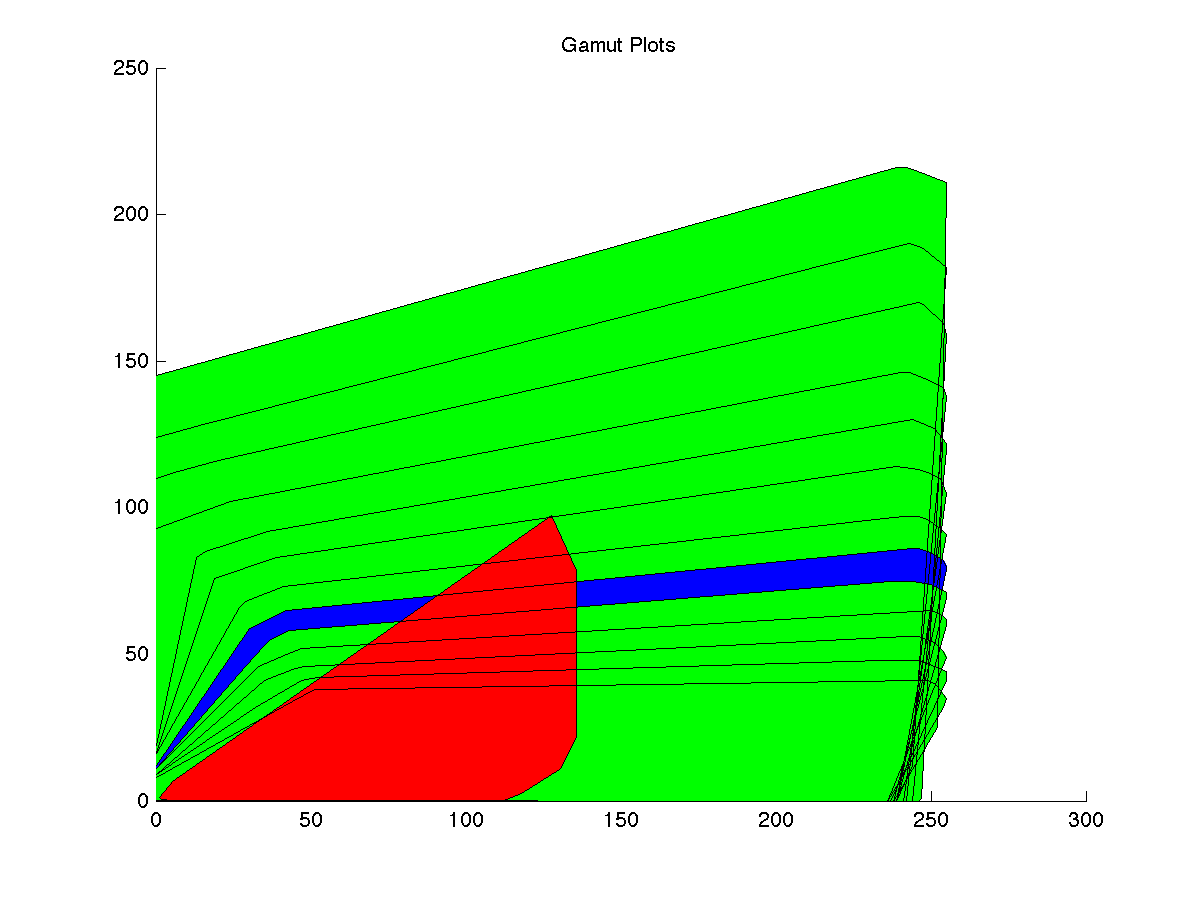
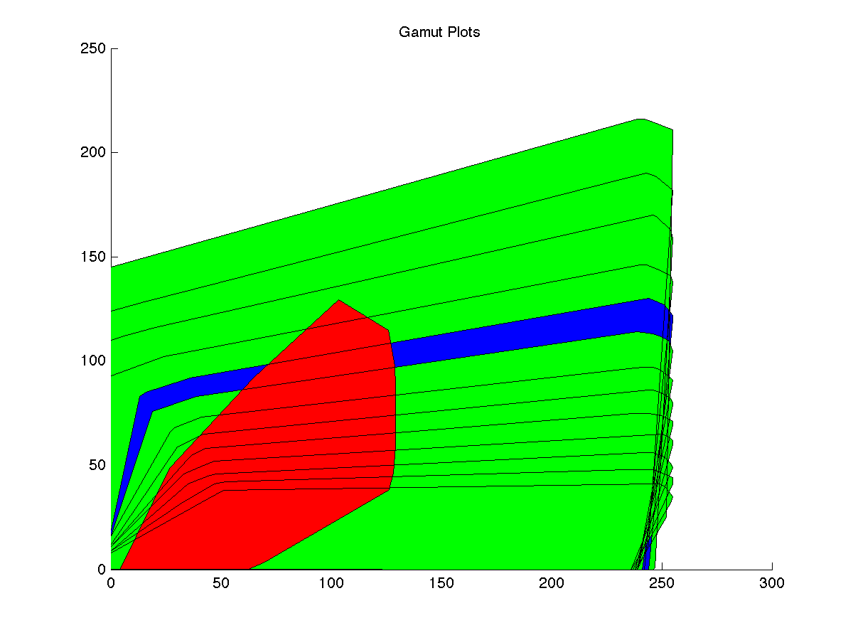
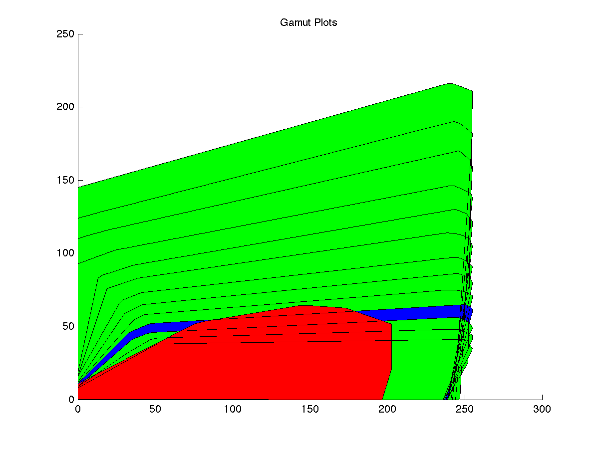
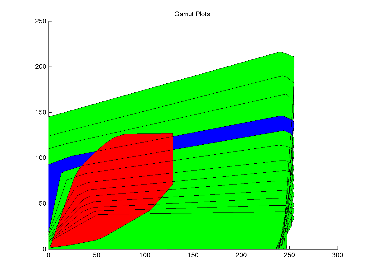
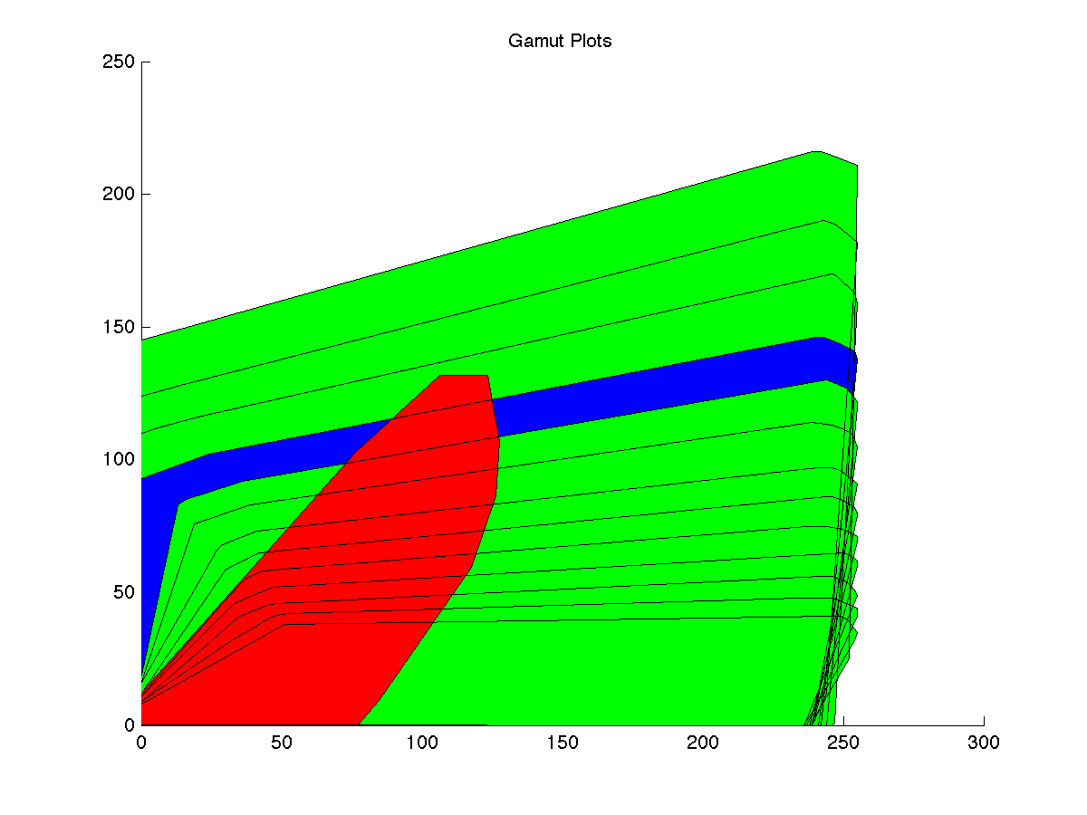
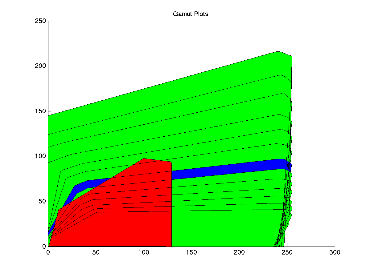
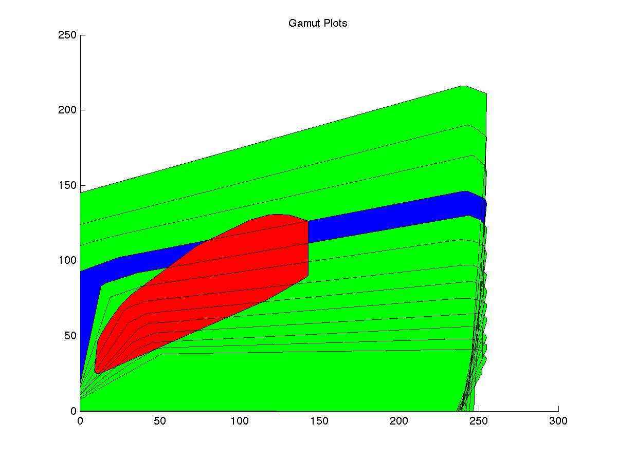
This is an illuminant estimation algorithm that differs quite dramatically from the previous methods because it requires detailed knowledge of one's imaging sensor. It is based on the idea that most photographs are taken in only a limited number of illuminant types. This is exemplified in the CIE’s set of standard illuminants for sun, incandescent, and fluorescent light. The range of colors that is possible in any scene is limited by the illumination. Sensor Correlation is a method that compares the color gamut in an image with those of many illuminants determined a priori by the responsivity of the imaging sensor. The reference gamut that correlates the most with the image gamut is determined as the most likely illuminant in the scene.

In my implementation, I simulated the reference gamuts using the MacBeth color checker in ISET under a black body radiator at 13 different temperatures, equally spaced on the mired scale. Note that this algorithm should be specific to each camera’s sensor but I nevertheless applied it to images whose origins were completely unknown. This is technically an incorrect usage but it examines the possibility of using an average set of reference gamuts that would be useful for a wide range of image sensors.

function sensorCorrelation(filename,outFile,catType,plots) %sensorCorrelation(filename,outFile,catType,plot) % Performs the sensor correlation method for illuminant estimation and then % a chromatic adaptation transform for correction. % Set plot = 0 or 1 to turn diagnostic plots on or off.

1. Pre-process to eliminate aberrant colors. This is described in more detail in the reference papers but it also involves normalizing the brightness of the image and getting rid of saturated colors. clipVal = 225; %% pre-process % simplify by ignoring pixels with any RGB value >= 225+1 since we will saturate later imRGB = imRGB(:,max(imRGB,[],1)<clipVal+1); % populate color space imRGBSpace = zeros(clipVal+1,clipVal+1,clipVal+1,'uint8'); for i=1:size(imRGB,2) c = imRGB(:,i); imRGBSpace(c(1)+1,c(2)+1,c(3)+1) = imRGBSpace(c(1)+1,c(2)+1,c(3)+1) || 1; end % compute connectivity lookup table, must have more than 1 neighbor imRGBSpaceConn = imfilter(imRGBSpace,conndef(size(imRGB,1),'maximal'))>2; imRGBConn = false(1,size(imRGB,2)); for i=1:length(imRGBConn) c = imRGB(:,i); imRGBConn(i) = imRGBSpaceConn(c(1)+1,c(2)+1,c(3)+1); end imRGB = imRGB(:,imRGBConn); %keep only pixels in the image with connected color values clear imRGBSpaceConn imRGBSpace imRGBConn %ignore pixels with any RGB value >= 225, saturated imRGB = imRGB(:,max(imRGB,[],1)<clipVal); % normalize I = zeros(1,size(imRGB_orig,2)); for i = 1:length(I) I(i) = norm(imRGB_orig(:,i)); %sqrt(R^2+G^2+B^2) end imRGB = 255*imRGB/max(I);;
2. Compute the color gamut of the remaining pixels as the convex hull of the red and blue channels. [gamut_im,gamutArea_im] = convhull(imRGB(1,:),imRGB(3,:)); [x,y] = poly2cw(imRGB(1,gamut_im), imRGB(3,gamut_im)); gamut_im = [x; y]; %the image gamut vertices
3. Correlate the image gamut (at a variety of scalings) with the reference response gamuts under different temperature illuminants. Choose the one with greatest correlation as our estimate of the color cast. kScale = .1:.1:1; %rows are scaling, cols are different illuminants corr = zeros(length(kScale),length(gamutArea_illum)); for j=1:length(kScale) k = kScale(j); for i = 1:length(gamut_temps) gi = gamut_illum{i}; [x,y] = polybool('&',k*gamut_im(1,:),k*gamut_im(2,:),gi(1,:),gi(2,:)); corr(j,i) = polyarea(x,y)/sqrt(gamutArea_im*gamutArea_illum(i)); end end [corr,k] = max(corr,[],1); [maxCorrVal,targetIllum] = max(corr); k = k(targetIllum); T = gamut_temps(targetIllum) %the estimated temperature of the illuminant
4. Use a chromatic adaptation transform to correct for the color cast and reach the D65 canonical illuminant %xyz color cast estimate normalized Y to 100 xyzEst = xy2XYZ(XYZ2xy(gamut_XYZ(:,targetIllum)),100); imRGB = cbCAT(xyzEst,xyz_D65,catType)*imRGB;

The gamut plots show the reference illuminant gamuts in green and the estimated illuminant gamut with highest correlation in blue. The image gamut is shown in red. Note that the reference gamuts are quite different than the ones presented in the papers. This might be because they were simulated by ISET rather than measured.

Clearly, the reference gamuts produced with ISET do not correspond well with the imaging sensor to take this photo. Now we see the effects of having an incorrect illuminant estimation.

ISET was used to generate an artifical color cast on the flower. The simulated illuminant temperature was 3268K. Sensor Correlation estimated the illuminant as 3034.9K. The image still develops a blue cast after correction even though this is a completely simulated application that should work. Perhaps the chromatic adaptation transform is not the proper method for correction.

Given that all the images develop blue cast after color balancing, I feel that there is something wrong with my implementation. It could be because I am using the wrong reference gamuts to almost all the photos but the simulted ISET flower photo should have worked then. This requires further debugging.