Color Balancing Algorithms | Illuminant Estimation | Gray World

Introduction

Gray world is among the simplest estimation methods. The main premise behind it is that in a normal well color balanced photo, the average of all the colors is a neutral gray. Therefore, we can estimate the illuminant color cast by looking at the average color and comparing it to gray.

Implementation: grayWorld.m

function grayWorld(filename,outFile,catType,maxIter,plots)
%grayWorld(filename,outfile,catType,maxIter,plot)
% Performs color balancing via the gray world assumption and a chromatic
% adpatation transform.  Can be run interatively to possibly improve the
% result.  Set plot = 0 or 1 to turn diagnostic plots on or off.

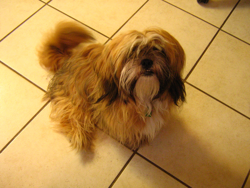
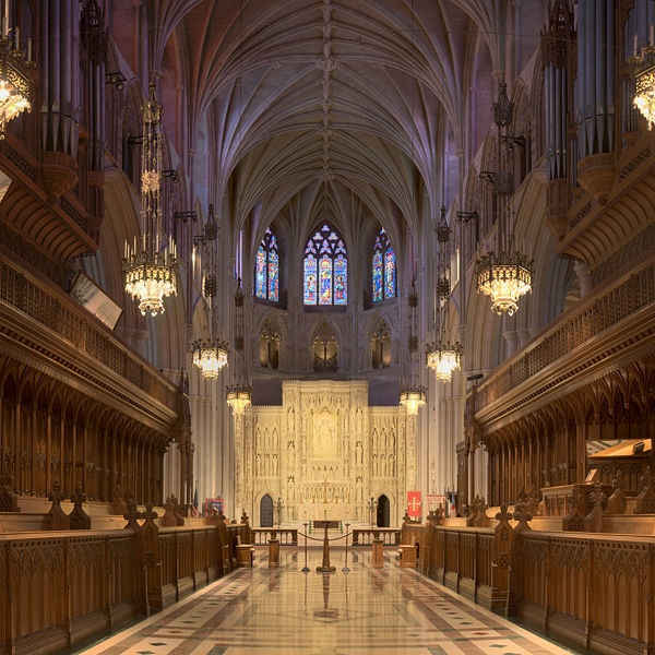
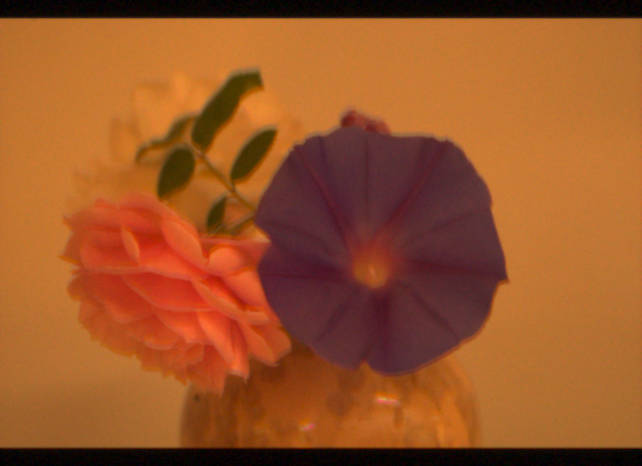
Estimate the color cast using the mean RGB value across the whole image. rgbEst = mean(imRGB,2);
Convert to xy-chromaticity then XYZ assuming the image already lives in the sRGB color space. The hope is that the manufacturer has made whatever conversions are necessary to put their sensor outputs in sRGB space when it stores JPEGs. xyEst = XYZ2xy(sRGBtoXYZ*rgbEst); %calculate xy chromaticity xyzEst = xy2XYZ(xyEst,100); %normalize Y to 100 so D65 luminance comparable
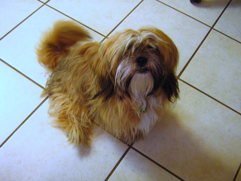
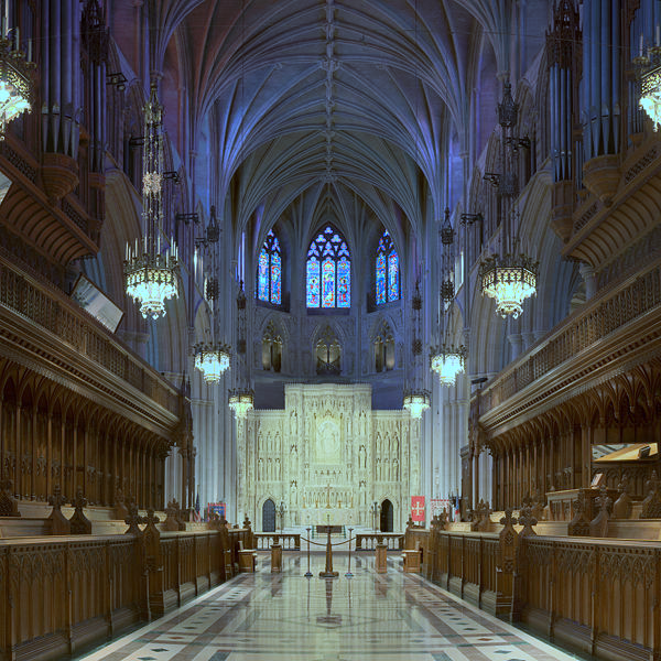
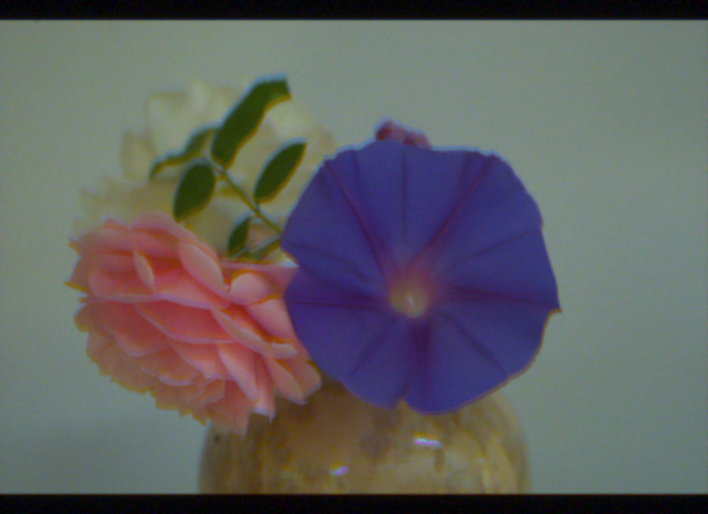
Apply a chromatic adaptation transform to reach the target D65 canonical illuminant. imRGB = cbCAT(xyzEst,xyz_D65,catType)*imRGB;

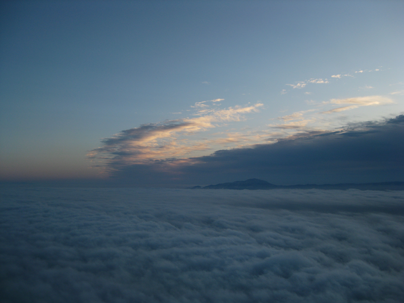
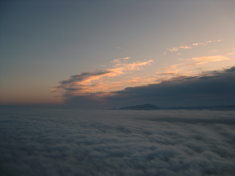
This process can be looped to try to force the average color to a neutral gray. Usually this is too extreme and is an indication that the gray world assumption is not correct in general. Consider a photo of the ocean, for example. Nevertheless, it provides a reasonable rough estimate of the illuminant.

Gray world does a decent job here. The tiles develop a blue tint though. The difference between CAT spaces is subtle with XYZ preserving more of the vibrant colors in the puppy's fur.