Introduction

There are a variety of methods to achieve adaptation but I looked at the most standard model, called von Kries's model or the chromatic adaptation transform. The underlying principle is that in order to change the apparent illumination of a photo, we need to excite the same LMS cone responses in the eye as with our desired illuminant. Typically, we assume that this is possible with a diagonal scaling of the axes after a transformation from XYZ to a space that more resembles the LMS cone space. In other words, once we're in the right space, we simply need to divide out our estimated illuminant and apply our desired illuminant separately for each channel. In matrix form this is represented as:

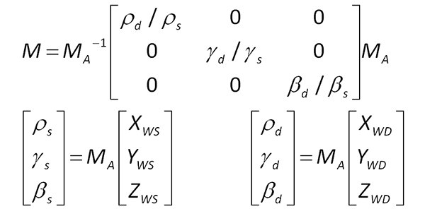
The choice of the transformation matrix, MA, is the subject of research [1]. It can be optimized to a variety of criteria, such as mean ΔEab or statistical distribution testing [5]. In any case, the goal here is to implement these different transformations and to gain some intuition about their performance.

Our desired lighting is the D65 CIE standard illuminant, which represents spectrum of the sun at mid-day. This is the white point for the sRGB color space that most monitors are calibrated for.

The available transforms are:
  • von Kries
  • Bradford
  • Sharp - based on sharpened sensors, min. XYZ errors
  • CMCCAT2000 - fitted from all available color data sets
  • CAT02 - optimized for minimizing CIELAB differences
  • XYZ

Implementation: cbCAT.m

function outMat = cbCAT(xyz_est,xyz_target,type) %outMat = cbCAT(xyz_est,xyz_target,type) % Chromatic adaptation transform via von Kries's method. % type chooses the LMS-like space to apply scaling in, valid options: % 'vonKries', 'bradford', 'sharp', 'cmccat2000', 'cat02', 'xyz' % See http://www.brucelindbloom.com/index.html?Eqn_ChromAdapt.html
  1. Set up transformation matrices. % the following are mostly taken from S. Bianco. "Two New von Kries Based % Chromatic Adapatation Transforms Found by Numerical Optimization." if strcmpi(type,'vonKries') %Hunt-Pointer-Estevez normalized to D65 xfm = [.40024 .7076 -.08081; -.2263 1.16532 0.0457; 0 0 .91822]; elseif strcmpi(type,'bradford') xfm = [.8951 .2664 -.1614; -.7502 1.7135 0.0367; 0.0389 -0.0685 1.0296]; elseif strcmpi(type,'sharp') xfm = [1.2694 -.0988 -.1706; -.8364 1.8006 0.0357; 0.0297 -0.0315 1.0018]; elseif strcmpi(type,'cmccat2000') xfm = [.7982 .3389 -.1371; -.5918 1.5512 0.0406; 0.0008 0.239 0.9753]; elseif strcmpi(type,'cat02') xfm = [0.7328 0.4296 -.1624; -.7036 1.6975 0.0061; 0.0030 0.0136 0.9834]; else xfm = eye(3); end
  2. Compute diagonal scalings from the estimated illuminant XYZ and D65 XYZ. gain = (xfm*xyz_target)./(xfm*xyz_est);
  3. Create the matrix M, then include transformations from sRGB to XYZ and back. outMat = xfm\(diag(gain)*xfm); sRGBtoXYZ = [0.4124564 0.3575761 0.1804375; ... 0.2126729 0.7151522 0.0721750; ... 0.0193339 0.1191920 0.9503041]; outMat = inv(sRGBtoXYZ)*outMat*sRGBtoXYZ;

Results

Gray World

The difference between CAT spaces is subtle. XYZ seems to produce a more saturated output. I think it's very difficult to judge which space is the most accurate and as far as my eye is concerned, it's a complete toss-up.

Robust Auto White-Balance with CAT

Sensor Correlation