Color Balancing Algorithms | Illuminant Estimation | Robust Auto White-Balance

Introduction [2]

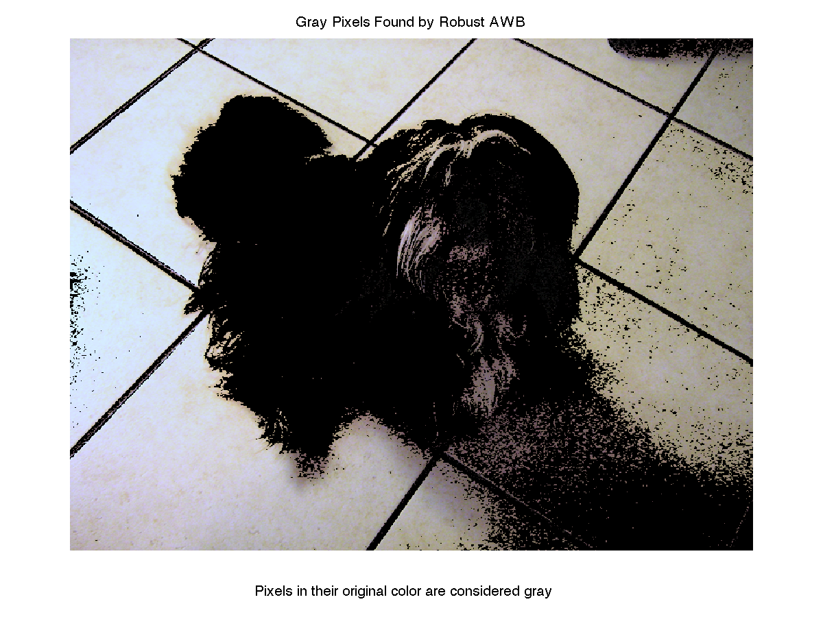
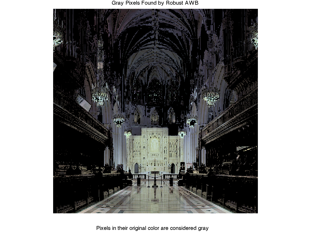
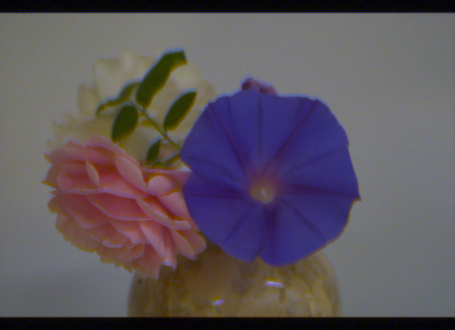
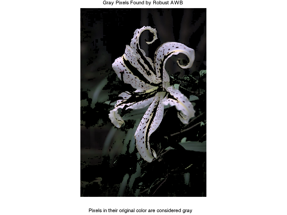
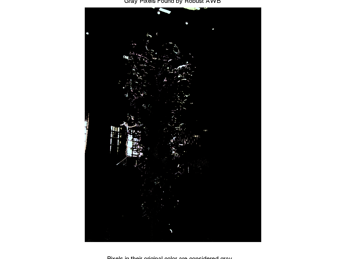
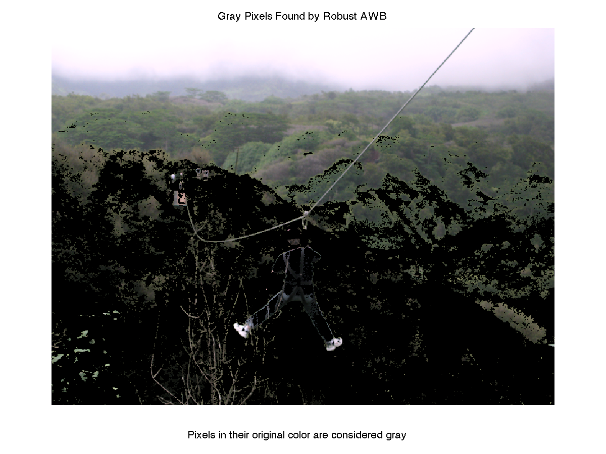
The technique presented by Huo et al. is essentially a more careful application of the gray world idea. Instead of averaging all the pixels in an image, the algorithm selects slightly off-gray candidates based on their YUV coordinates that are more likely to reveal information about the scene illuminant rather than the object's own color. The choice of the threshold for what is acceptably off-gray is a parameter that can be tweaked. Values around 0.3 are typical.

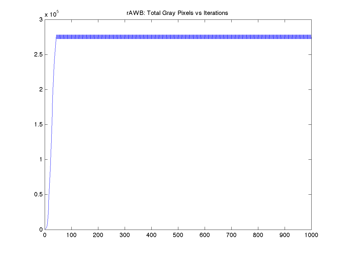
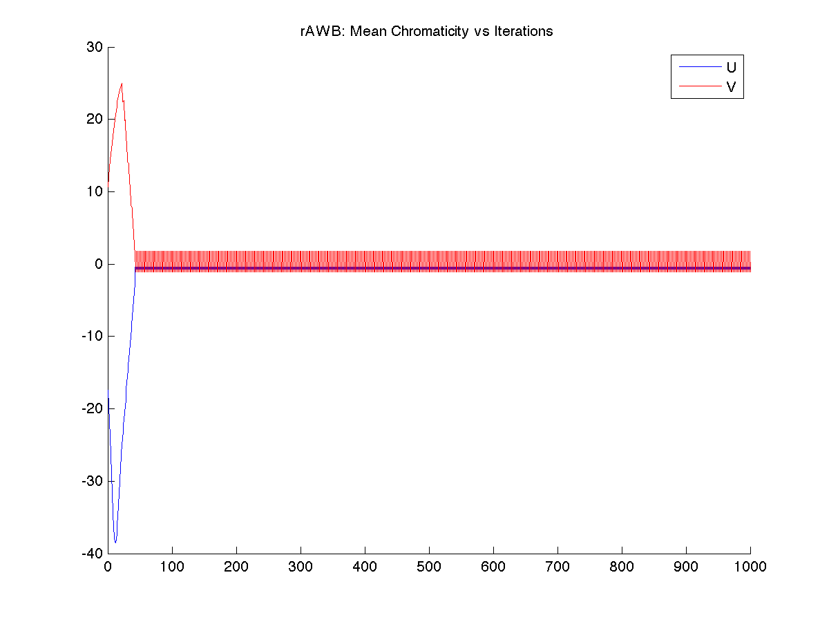
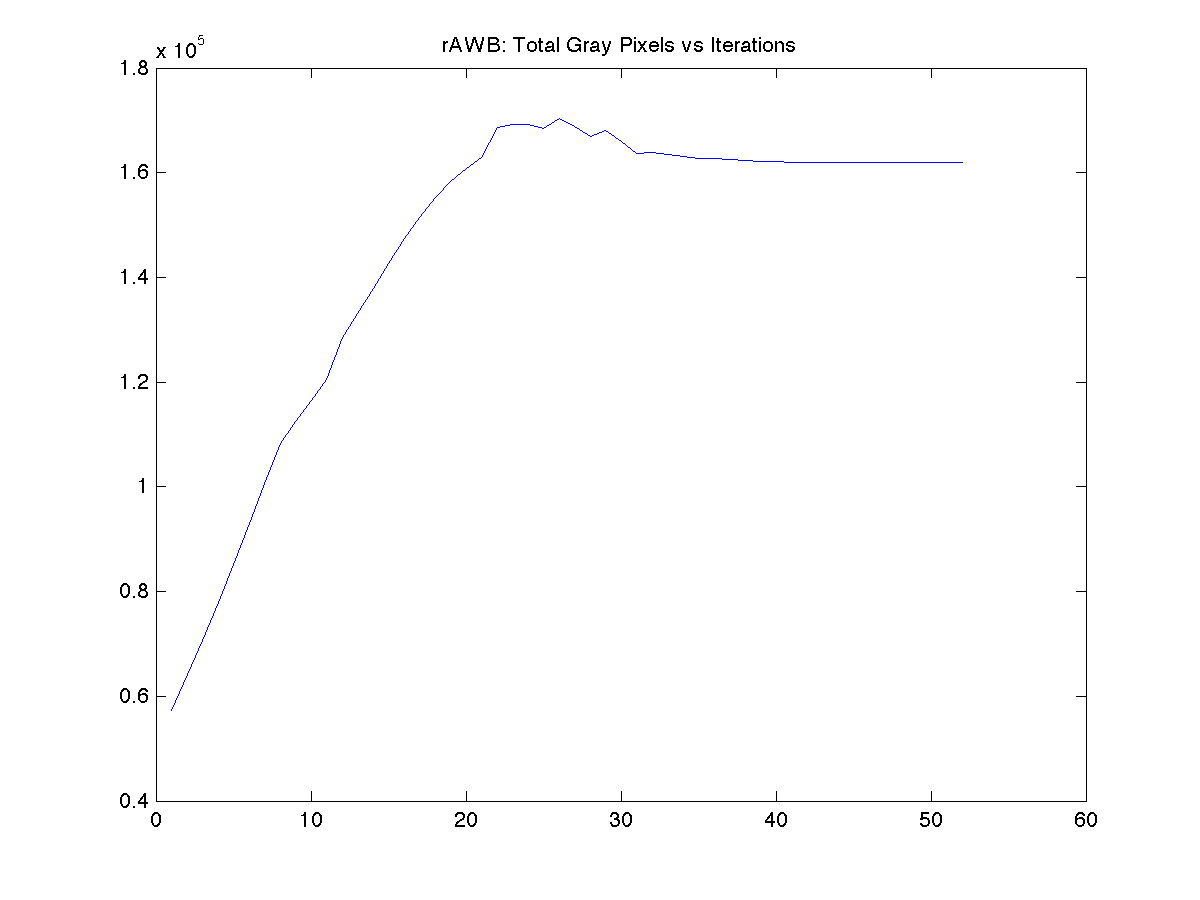
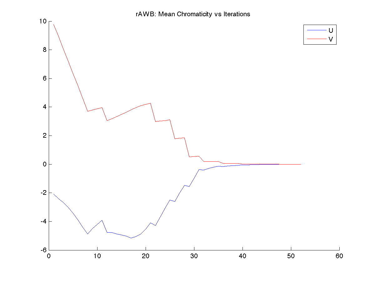
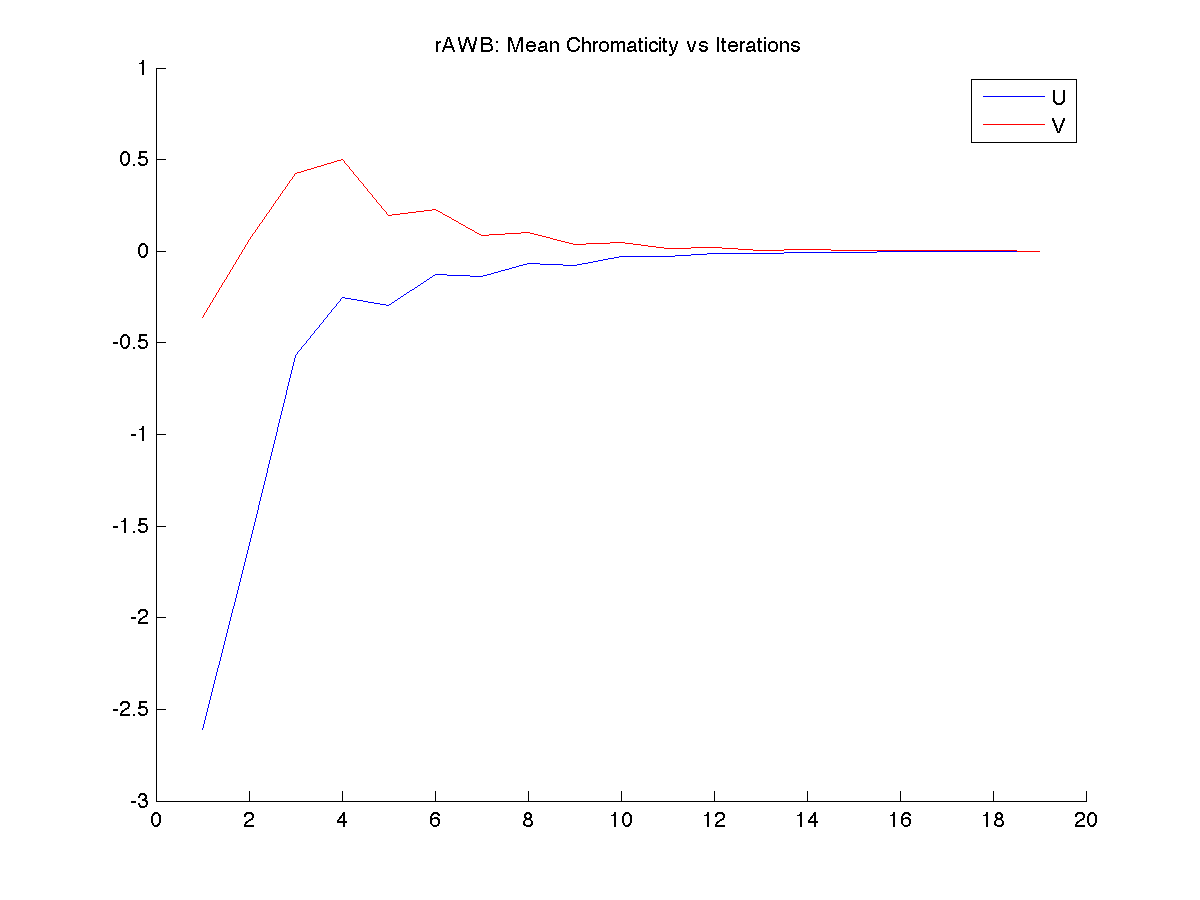
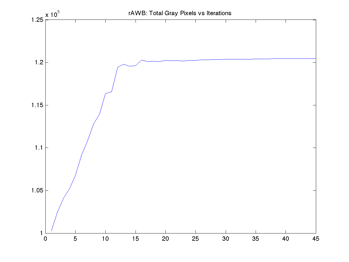
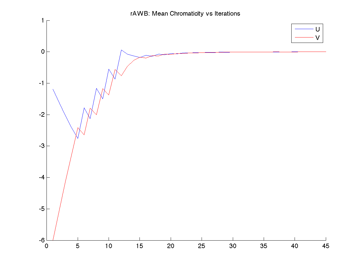
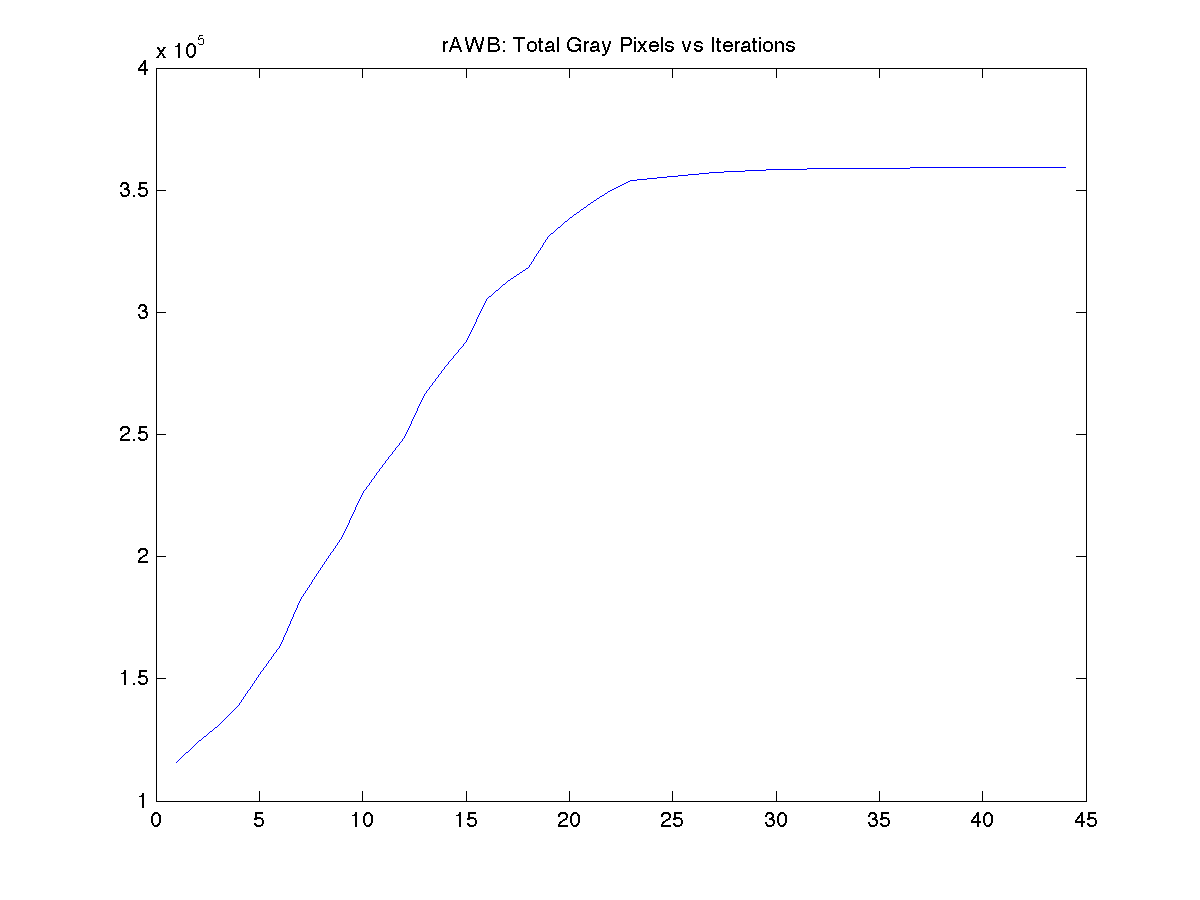
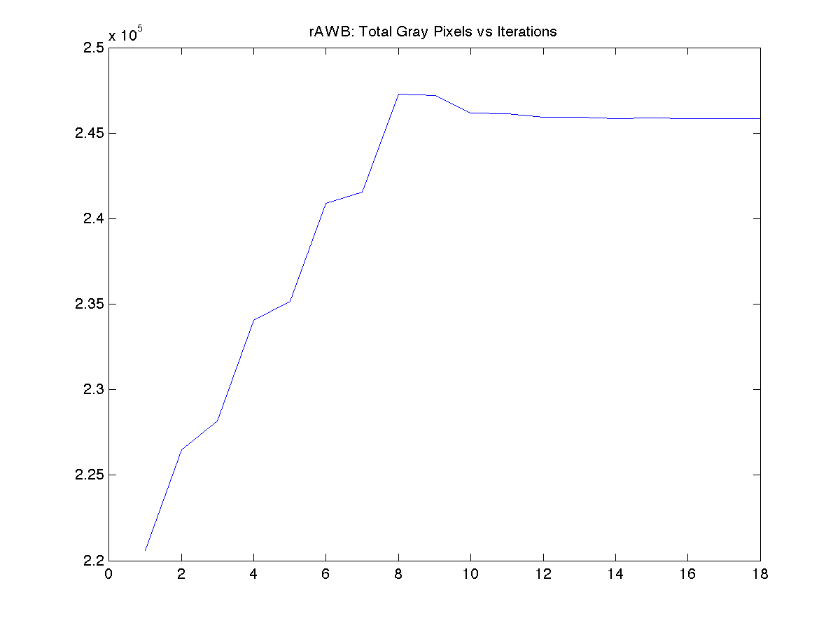
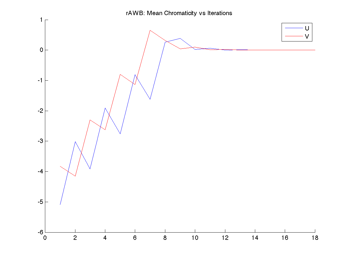
This method was designed for video cameras in mind where one would like to achieve color balance in a few frames. It is meant to be implemented in hardware where changing the gain of channel responsivities is easy. A negative feedback loop is used in the algorithm to try to drive the off-grays to complete neutral gray. Despite this, I have adapted it for photographs at the price of a longer processing time than the other algorithms I implemented.

Implementation: robustAWB.m

function robustAWB(filename,outFile,option,catType,T,maxIter,plots)
%robustAWB(filename,outFile,option,catType,T,maxIter,plot)
% Performs robust auto white-balancing by estimating gray pixels based on
% their deviation in YUV space then applying an iterative correction via
% CAT or directly adjusting the R and B channels.
% Set option = 'RB gain' or 'cat' for the correction method.
% Set T higher for a larger threshold of deviation to consider off-gray.
% Set plot = 0 or 1 to turn diagnostic plots on or off.

Convert to YUV color space. xfm = [0.299 0.587 0.144; ... -0.299 -0.587 0.886; ... 0.701 -0.587 -0.114]; im = xfm*imRGB; %convert to YUV
Estimate illuminant by finding pixels that are similar to gray within a threshold: (|U|+|V|)/Y < T F = ( abs(im(2,:)) + abs(im(3,:)) )./im(1,:); grays = im(:,F<T); U_bar = mean(grays(2,:)); %estimate of the U of the illuminant V_bar = mean(grays(3,:)); %estimate of the V of the illuminant rgbEst = inv_xfm*[100;U_bar;V_bar]; %convert the average gray from YUV to RGB xyEst = XYZ2xy(sRGBtoXYZ*rgbEst); %calculate xy chromaticity xyzEst = xy2XYZ(xyEst,100); %normalize Y to 100 so D65 luminance comparable
Apply adaptation. The original method was to adjust the gain on the R and B channels because these are the ones primarily affected by a illuminant color cast. For example, in a sunset scene, the red channel is very bright so its gain should be lowered. However, this makes more sense in a hardware application. I had the idea of applying a chromatic adaptation transform (CAT) instead.
- R/B gain: Either the red or blue channel is adjusted according to the illuminant estimation. We quit if we're close enough to neutral gray. % gain adjustment parameters, can probably be optimized via more control system analysis u = .01; %gain step size a = .8; %double step threshold b = .001; %convergence threshold if abs(U_bar) > abs(V_bar) % U > V; blue needs adjustment err = U_bar; ch = 3; %blue channel else err = V_bar; ch = 1; %red channel end if abs(err) >= a delta = 2*sign(err)*u; %accelerate gain adjustment if far off elseif abs(err) < b %converged delta = 0; disp(['Converged. U_bar and V_bar < ' num2str(b) ' in magnitude.']) break else delta = err*u; end gain(ch) = gain(ch)-delta; %negative fdbk loop imRGB = diag(gain)*imRGB_orig;
- CAT: With an estimate of the illuminant, we can convert to XYZ and then apply a CAT to get to our D65 canonical illuminant. if max(abs([U_bar V_bar])) < b disp(['Converged. U_bar and V_bar < ' num2str(b) ' in magnitude.']) break elseif iter >= 2 && norm([U_avg(end)-U_avg(end-1) V_avg(end)-V_avg(end-1)]) < 10^-6 disp(['U_bar and V_bar are no longer improving.']) break end rgbEst = inv_xfm*[100;U_bar;V_bar]; %convert the average gray from YUV to RGB xyEst = XYZ2xy(sRGBtoXYZ*rgbEst); %calculate xy chromaticity xyzEst = xy2XYZ(xyEst,100); %normalize Y to 100 so D65 luminance comparable imRGB = cbCAT(xyzEst,xyz_D65,catType)*imRGB;
Loop until the average of the off-gray points converges to a neutral gray or until we are no longer improving.

There are convergence/instability issues for this highly orange tinted image. The performance is quite decent though. The usage of a CAT instead of adjusting R/B gains provides some benefit in preserving color saturation.