PSYCH 221 FINAL PROJECT

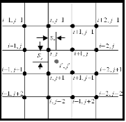
The first straigthforward approach was to interpolate. We began by trying several commonly used interpolation schemes: bicubic, tricubic, hermite, and spline. We then discovered a paper on image resampling using an adaptive bicubic method, local feature bicubic interpolation:

Bicubic/Tricubic

Hermite

Spline

Bicubic/Tricubic:

Cubic interpolation is one of the most common interpolations schemes since it is the simplest interpolation method that "offers true continuity between the segments."[2] 2 The 1D cubic interpolation formula for estimating the value between y1 and y2 is seen above. To apply this formula in two directions, x and y, independently, bicubic interpolation is performed. To attempt to get even more precise interpolation the formula can be applied not only to the x and y direction but also across the diagonals, tricubic interpolation.

Local Feature Based Bicubic Interpolation:

Adaptive Image Enlargement

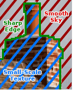
Reading the literature we found that there are both non-adaptive and adaptive interpolation schemes. The adaptive interpolation schemes attempt to factor in whether the surrounding pixels represent an edge, smooth flat region, or a textured area. These adaptive interpolation methods we found are proprietary and designed for image enlargement. One scheme we came across attempted to use the local features to adapt the bicubic interpolation method. They understood that the bicubic interpolation method has a blurring problem. Therefore, they used the local asymmetry of the features and the local gradient of the surrounding pixels to remove this blurring in their own interpolation method. There were three stages to their solution. The first stage used the local asymmetry of the image features, but failed because it performed poorly with peaks and troughs. The second stage used the local gradient but failed because it sometimes overshot the interpolated pixel value. Therefore, finally they combined both approaches to mitigate each stages problems and come up with a ‘superior’ solution that did remove the blurring problem of the bicubic interpolation method.

Hermite:

Hermite interpolation is very similar to cubic interpolation in that it requires four points and offers high degree of continuity between the points.
What makes this interpolation method unique is that it has additional parameters that allow you to adjust the tension and biasing. The tension parameter allows the curvature between points to be tightened up. The biasing parameters allows curve to twist around the given points. The tension parameters can vary between 1 and -1 (high and low tension). The bias parameter can vary largely but is 0 if the desired interpolation is to provide even bias between given points on the left and right.

Spline:

Background and Theory:
Spline interpolation uses low-degree (in our case 3rd degree) polynomials between data points. It chooses the polynomial pieces such that they fit smoothly together.
Difference between Qubic – Spline and normal polynomial interpolation:
It is not always possible to find a polynomial, which interpolates all data points. Splines are piece-wise defined functions whose individual curves meet at data points [7]. An example of how Spline and a 11th degree polynomial performs is the following [8]:

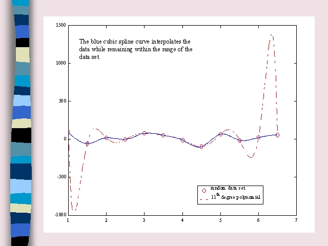
As can be seen, the 11th degree polynomial makes huge jumps after the first and before the last point which adds to the error profile of the interpolation scheme.
To make use of this feature of spline, we implemented the following spline interpolation for our image:
As known, we have two missing rows. We interpolate every nth pixel along those rows horizontally via spline technique. This means we take every nth column of the image and each column has two pixels missing. We interpolate those two pixels via the spline algorithm. After finding those pixels in every nth column of the image, we form two separate arrays out of those pixels, one of the first missing row and the other for the second missing row. At this point, we have the following picture:

170 corresponds the value found for the first column. 155 corresponds to the value found for the (n+1)th column. Now, we have n (5 in the above case) values to interpolate. Here, we exploit the piece-wise feature of the spline since we might not be able to find a polynomial, which interpolates every known data points.