Test Implementation:
To evaluate our algorithms we used the methodology described in the testing and performence metrics section. We ran each algorithm over 10 randomly selected double rows in two images, one with high SNR and the other with low SNR. Hence, we tested each algorithm over 20 instances and used the acquired error data to generate the attached figures.
Histograms of Delta E error distribution:
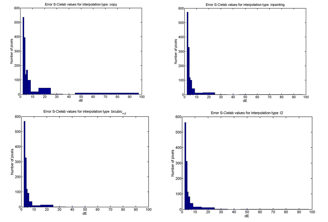
Looking at the histograms of delta E error distributions, we find several worthy points to establish. First, there is a significant reduction in the delta E errors compared to they copying method for all the methods shown in the results. Second, the convex L2 method produces the least number of errors in range of 10-20 delta E. However, it produces more errors in the 20-30 delta E range than Inpainting or Bicubic with Gaussian filter. It should be noted though that there are only a couple of errors produced in this range. Third, using a filter with interpolation method works just slightly better than using Inpainting across the entire range of errors. The reason maybe because there is only one stage for processing in Inpainting to interpolate, whereas interpolation with a filter has two stages for processing. The filter stage may reduce the artifacts resulting from typical interpolation methods such as aliasing, edge halo, and blurring.
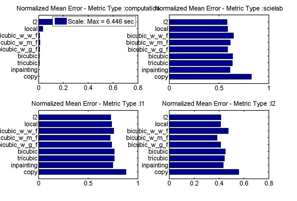
The bar graphs for computation time and mean error show us on average how we can compare how these methods that perform over a wide range of images and missing lines. In terms of mean error (delta E, L1 Norm, or L2 Norm) all the methods perform very closely. Looking very carefully, we see that the best methods in terms of reducing mean delta E, are convex L2, interpolation with filters, and Inpainting. As expected, we found that adding a filtering stage after interpolation improved results as seen in experiments for reducing line scratches in archived film.
It should be noted that the Wiener filter did not work very well compared to the Gaussian and Median filter (in terms of delta E). This suggest that Wiener filter, commonly used to reduce power noise degradation, was not a suitable match to model the degradation differences between the interpolated image and the original image. The Gaussian and Median filters were better than each other depending on the image used. For example, the Median filter probably outperformed when there were edges since the Median filter is better than the Gaussian filter at preserving edges.
Inpainting's advantage over the interpolation methods with filters seems to be that it requires the less computation time. Convex L2's disadvantage seems to be that it requires a significant computation time, approximately 6.5 seconds on average. This computation time is a magnitude higher than all other methods tested. It will be noted that computation could have been reduced significantly if given more time to work on the project. For example, one could use specific techniques such as block elimination to exploit the structure in the images to reduce the computation time. Also, these computation times are very rough and include the interpreting overhead in MATLAB. If further explored, this computation could be reduce to the goal of 2-3 seconds. Finally, we'd like to note that in these bar graphs there is an error level that cannot be beat. Some information has been lost in image capturing and can never be recovered. A good follow on analysis of this project would inspect the smallest error possible using all the information in the image for interpolation.
Taking our initial goals back into perspective we find that Fairchild could proceed with several of these schemes. In particular, further exploration should be taken in the following methods: multiple interpolation methods/filters in series, Inpainting, and Convex L2. The multiple methods in series could explore using several interpolation methods such as bicubic, hermite, and sinc interpolation in series. Computationally, there should be no issues placing a couple more methods in series. Image inpainting has the disadvantage of performing more slowly when applied to bigger images with more missing rows and more columns due to its linear nature. The core of the algorithm, propagating information to the target region from the neighbor pixels, helps it achieve small error performance. Further improvements might include choosing a bigger neighborhood region for the target pixels and introducing new coefficients for the new neighbor pixels consistent. However, there is a trade-off between choosing a bigger region and computation time; therefore, more work can be done to find the optimal size for the neighborhood region. Convex L2 could be promising since it reduces large errors the 'best.' If it was optimized we believe, the computation time could fall under the goal of 2-3 seconds.
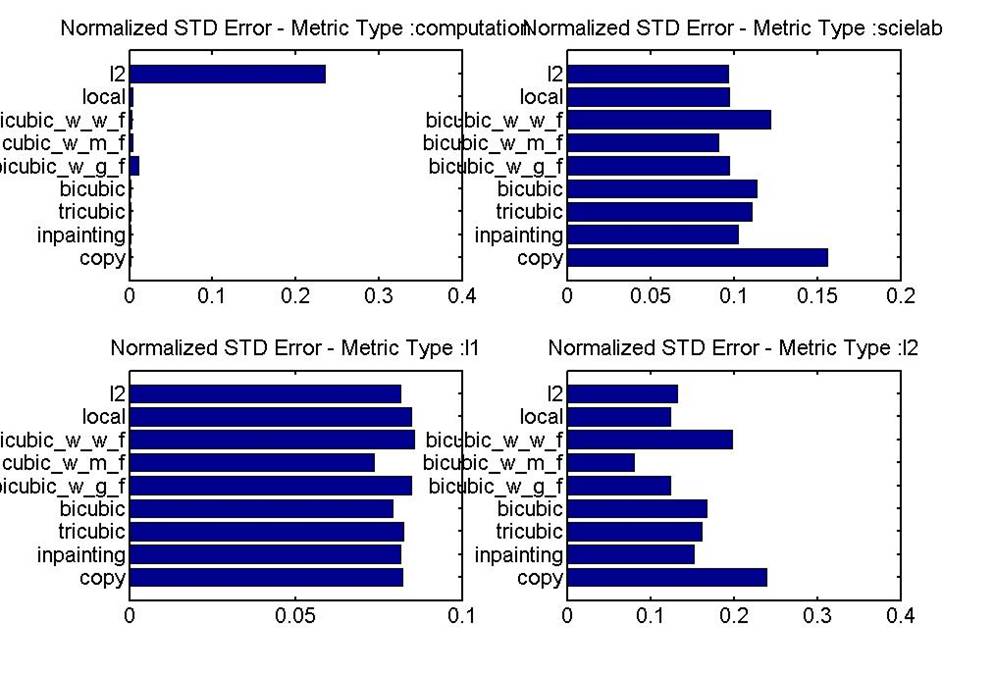
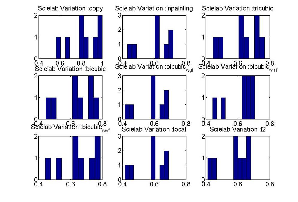
Below are the graphs of computation time/mean error, computation time/std error, variation across images:
|