[ Main ] [ Outline ] [ Introduction ] [ MRI Basics ] [ Cross-Relaxometry ] [ Results ] [ References ] [ Appendix ]

Magnetic Resonance Imaging (MRI)

Magnetic resonance (MR) is a quantum mechanical phenomenon. It relies on the property of some atoms to have magnetic dipole moments. When placed in a strong magnetic field (B₀), the magnetic dipoles align with the field, creating a net magnetization in the direction of B₀. Once aligned, the magnetic dipoles are not static. They oscillate around the static field with a frequency known as the Larmor frequency as shown in Figure 1. The Larmor frequency (ω) is proportional to the strength of the static field, and the proportionality constant is γ.

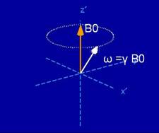
Figure 1. Free precession of a spin around a static magnetic field (figure courtesy of Brian Hargreaves)

One atom with a dipole moment is the hydrogen atom (proton) which is found in abundance in the human body, both in water and in more complex molecules. When placed in a strong magnetic field, the hydrogen atoms generate a net magnetization in the B₀ direction, precessing at the Larmor frequency. However, as long as the magnetization is constant, there is no way to obtain a signal that will depend on the structure of the human body. In order to make the oscillation dependent on the tissue structure, there needs to be a temporal and spatial variation of the magnetization vector.

The way to obtain temporal variation is by applying a time-varying RF (radio frequency) magnetic field, at resonance with the Larmor frequency. Applying the RF field at resonance will result in the tipping of the net magnetization vector M away from the axis of rotation, and into the transverse plane x-y.

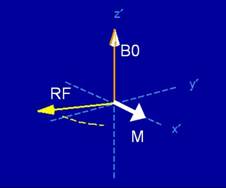
Figure 2. Applying an RF pulse centered at the Larmor frequency causes the magnetization vector (white arrow) to tip into the transverse plane (figure courtesy of Brian Hargreaves)

The way to obtain spatial variation is to apply magnetic field gradients, that will make the static magnetic field vary across the region of interest. By varying the frequency and orientation of the oscillation of the hydrogen atoms in the human body, it is possible to obtain an electric signal dependent on the location of the hydrogen atoms. If the magnetization in different parts of the region of interest precesses with a different frequency, we get a unique precession frequency to spatial location mapping.

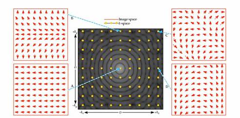
Figure 3. The figure above illustrates the data acquired during an MRI acquisition. Each point in the acquired data results in a different spatial frequency, so the acquired data is a Fourier Transform of the object imaged (courtesy of Huettel et al.)

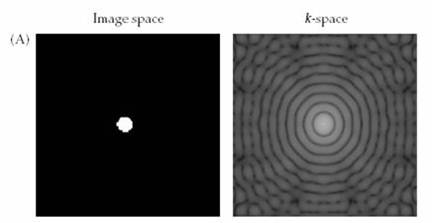
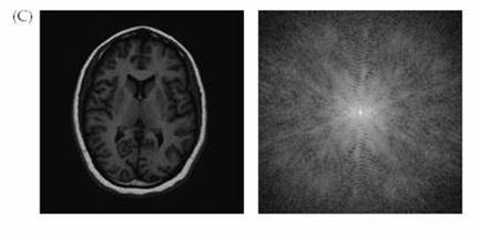
Figure 4. Image and k-space. The data from the scanner is k-space data. The image space data is a Fourier transform of the k-space data. (Figures courtesy of Huettel et al.)

As can be seen from the stated above, an MRI imaging sequence consists of excitation (tipping the magnetization in the transverse plane), traversal of k-space to obtain spatial frequency information, and transforming the k-space data to obtain the desired image. Since the timing of these operations is very important, and MRI imaging sequence is usually summarized in a timing diagram, that shows the order in which the excitation and the k-space traversal is performed. Such a timing diagram is shown below:

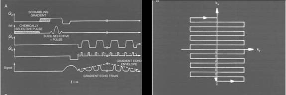
Figure 5. A timing diagram for an EPI (echo-planar imaging) sequence. The gradients (Gx, Gy, Gz) determine the speed with which k-space is traversed. In this timing diagram, when Gy is on, k-space is traversed horizontally, when Gx is on, k-space is traversed vertically. (Figure courtesy of Mansfield et al.)

Contrast Mechanisms

Once the magnetization is in the transverse plane, the RF pulse is turned off, and the magnetization slowly returns parallel to the B₀ field. The loss of magnetization in the transverse plane is called T2 decay, whereas the recovery of the magnetization along the z-direction is characterized by a time-constant T1.

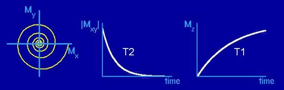
Figure 6. Illustration of T1 and T2 decay. Once tipped into the transverse plane, the magnetization vector decays in the transverse plane with time constant T2, while recovering along the z-axis with time constant T1 (figure courtesy of Brian Hargreaves)

It turns out that different tissues in the human body have different T1 and T2 time constants. As illustration, take a look at the picture below. It turns out that white matter in the brain has a shorter T1 than gray matter. Since the white matter magnetization recovers faster then the magnetization of the gray matter, the white matter in a T1-weighted scan of the brain will appear brighter than the gray matter.

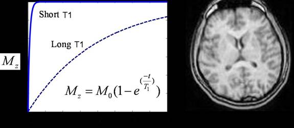
Figure 7. Illustration of T1-weighted contrast. Tissue with a short T1 constant appears bright (white matter in figure to the right). (Graph courtesy of Brian Wandell)

In addition to the T1 and T2 parameters, there are other contrast mechanisms that can characterize tissue, such as protein density, bound pool fraction and cross-relaxation rate. The last two are a result of a phenomenon called magnetization transfer.

Magnetization Transfer

As mentioned before, hydrogen in the human body can be found in water (liquid pool), but also in more complex molecules, such as proteins and lipids (macromolecular pool). For the T1 and T2 contrast, the RF pulse was applied on resonance, equally exciting the hydrogen atoms in the liquid and the macromolecular pool. However, if the RF pulse is applied off-resonance (usually off by several kHz), then the liquid pool in the region of interest remains unexcited, but the bound pool feels the off-resonance excitation [5,6].

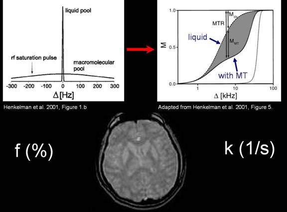
Figure 8. Illustration of MT contrast. The graph on the right describes the three categories of magnetization pools. The bottom (solid) line corresponds to a nearly completely saturated macromolecular pool. The middle line is the partially saturated liquid pool susceptible to magnetization transfer, whereas the top line is the liquid pool that is not susceptible to MT, which will appear the brightest on the MT image (bottom)

As a result, the liquid pool of protons will appear bright, whereas the macromolecular pool will be saturated by the off-resonance RF pulse, and will therefore appear dark. Therefore, the brightness will depend on the bound pool fraction, or the f parameter, defined as the molar fraction of bound protons. The tissue with high f will appear darker, because it will get saturated by the off-resonance pulse.

It turns out that not all liquid pool protons are equally immune to the magnetization of the macromolecular pool. Some liquid pool protons receive part of the magnetization from the bound pool, and this phenomenon is referred to as magnetization transfer. Since the rate at which magnetization is transferred from the macromolecular to the liquid pool is different for different protons in the liquid pool, this rate (called k, or the cross-relaxation rate) becomes another contrast parameter. The liquid pool with a faster cross-relaxation rate will appear darker because it will receive some of the saturation of the bound protons faster.

It is important to notice that for all these contrast mechanisms, we do not need an absolute value for T1, k and f in order to be able to obtain an image. In order to differentiate between tissues, it is good enough to get a relative mapping of those parameters, without precisely quantifying them.