[
Main ] [ Outline ] [ Introduction
] [ MRI
Basics ] [ Cross-Relaxometry ] [ Results ] [ References
] [ Appendix
]
Cross-Relaxation Imaging
with MR
In order to estimate the k and f parameters that we are interested
in for characterization of the brain tissue, we used a method known as cross-relaxation
imaging. A broad discussion of the theory and implications of the method can be
found in a paper by Yarynkh and Yuan [1]. The method
consists of two steps where we acquire data from the patient. Using theoretical
models explaining the behavior of our measurements [1,4,7],
we try to estimate some unknown parameters of interest.
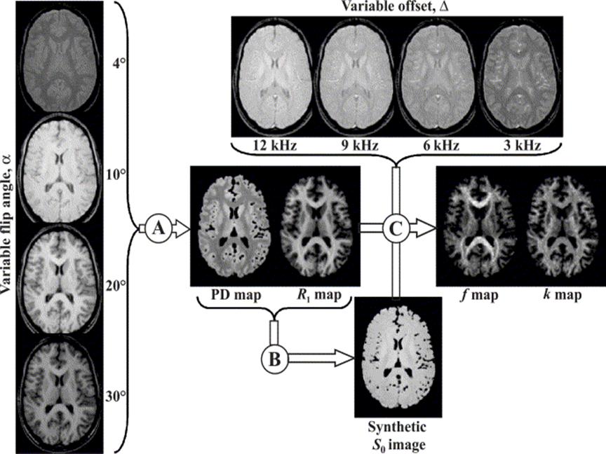
Figure
1. Diagram of k and f map
generation.
Figure 1 displays a summary of the outflow of the process. In the
first part, we acquire data with four different flip angles and using these
data we create PD and R1 maps (this step is labeled as A
in Figure 1). In the second part, instead of changing the flip angle to get
contrast in the measured data, we use a magnetization transfer pulse. By
varying the offset frequency at which the pulse is applied, we get four
different-contrast images. Using these data and the previous estimation
results, we are able to generate k and f maps (this step is labeled as C in
Figure 1). The creation of the synthetic image shown with letter B in Figure 1
is required for normalization purposes, to increase statistical stability of
the estimation process. The details of the estimation steps are explained in
later sections.
Pulse Sequence Selection
The pulse sequence selection is important
for the estimation process, as it is directly going to effect our signal
equations and the complexity of the estimations. We used a three-dimensional
(3D) spoiled gradient recalled acquisition in steady-state (SPGR) sequence for
data acquisitions. A basic pulse sequence diagram for 3D-SPGR is shown in
Figure 2. In an SPGR sequence the transverse magnetization is destroyed by
non-periodic phase changes in the RF pulse at each period (given by TR, repetition
time). Therefore the magnetization for an SPGR sequence can be represented as a
scalar rather than a three-dimensional vector in space. This property of SPGR
makes it suitable for estimation problems.
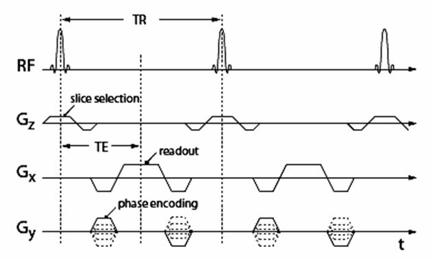
Figure
2. Pulse sequence diagram for an SPGR
sequence.
The reason for doing a 3D acquisition is
fast volume coverage within short scan times and higher signal-to-noise ratio
(SNR) that it provides. Short scan times make the data acquisition part of the
process feasible as you cannot keep the patients for long periods of time in
the scanner. SNR considerations are also important because we want to have a
small amount of noise for minimizing our estimation error. Finally, a 3D
acquisition with SPGR saturates signal coming from fresh-blood inflow, thereby
blood itself does not appear bright in the images.
The sequence used for the experiments is a
GE product sequence, Vascular TOF-SPGR. Data acquisition was performed on a
1.5T GE Signa 12X scanner with CV/i gradients. Two
different protocols were used for imaging. For the acquisition with varying flip
angles, TE = 2.4ms, TR = 20ms was used, while the flip angle had four different
values 4o, 10o, 20o, 30o. For the
second set of acquisitions, the flip angle was kept constant at 10o,
to minimize the T1 weighting in the acquired images. However, an additional
Fermi-shaped magnetization transfer pulse with 8ms duration and 670o
flip angle was added. TE = 2.4ms and TR = 32ms were prescribed. For both
acquisitions a matrix of 256x160x70 was used, where axial slice selection and
anterior to posterior readout direction were applied. To minimize the
acquisition time in the phase encode direction, half-Fourier encoding was
carried out, reducing the total samples to 80 in that direction. The
acquisition was completed in a single slab without any inter-slab overlap
slices. The acquisition resolution of 1.4mm x 2.3mm x 2.8mm,
was interpolated to 1.4mm x 1.4mm x 2.8mm during the scanner reconstruction.
Later the DICOM images were interpolated to isotropic 1.4mm resolution. The
auto pre-scan settings from the first data acquisition were kept the same
through a manual pre-scan before each acquisition.
T1 Estimation
The T1 estimation problem consists of getting
measurements with different flip angles ant using the theoretical signal
equation shown below to find a fit for T1 on a pixel basis. The signal S is a
function of the flip angle α, the repetition time TR, T1 and a
multiplicative factor in front named as PD. In fact, PD is a multiplication of
many factors itself which can all be grouped into one parameter for our
purposes. The flip angle and the repetition time are already known. Therefore
we have two unknowns.
The fitting is done with linear regression
analysis as explained by Fram et al. [8]. The signal
equation can be rearranged into a form that closely resembled a line equation
where the exponential term exp(-TR/T1) is the slope.
The term on the right with the factor PD in it, is a weak function of T1 and
therefore can be assumed to be a constant.
MT Fitting
The MT fitting problem is much more
complicated than the previous estimation problem as it involves the interaction
of bound and free pool protons, leading to matrix equations. The magnetization
vectors for both bound and free protons are given below, where each of the
terms are matrices themselves. Even when the equations
are scalarized the magnetization of free pool protons, which the directly
measured quantity in MR experiments, is a non-linear function of many variables
as seen. The flip angle and the offset frequency are preset by the user.
Estimates for PD and T1 are obtained in the previous step. However, we are left
with 5 unknowns.
In this form, the estimation problem is
very complex and many measurements have to be made in order to get estimates
for all of the parameters. This will increase the scan time beyond the practically
acceptable limit. Therefore, an appropriate approach is putting in average
values for some of the parameters that we are not directly interested in. T1B
cannot be measured at all, and in generally assumed to be 1s. T2B
has an average value that has little variation from person to person, which is
about 11us. Finally the ratio of T2 to T1 of free pool protons in the brain has
an average value of 0.055; we can use this ratio and our T1 estimates to figure
out what T2 is. In the end, our problem is reduced to a two-unknown problem
where the unknown are actually the parameters that we want to measure.
Once the MT measurements are completed,
the brain extraction tool (BET) by [9],is used to crop
out the extra-cranial tissue, followed by a T1 thresholding
( > 2s ) carried out to remove CSF from the images. A synthetic image that
reflects the signal that should have been detected at a TR of 32ms without any
magnetization transfer pulse is created using the PD, T1 maps obtained and the
signal equation for SPGR in the absence of magnetization transfer. This step is
important for increasing the statistical stability of the non-linear estimation
process to be carried out. K and f maps are created using MATLAB implementation
of the Levenberg-Marquardt [10] algorithm.