Single-Pixel Imaging

      The single-pixel camera developped at Rice University is an example of how compressive sensing allows us to move from a "Digital Signal Processing" (DSP) paradigm to a "Computational Signal Processing" (CSP) paradigm (Takhar, 2006). In this new paradigm, analog signals are no longer sampled periodically, but they are converted to a new representation, on which further processing is based.

      Apart from being an example of compressive sensing, such a single-pixel camera is also arguably useful when the detector is expensive and N-pixel arrays cannot be built. Time-multiplexing a single detector is then a cost-effective solution. For example, silicon is blind in the infrared, so CCD and CMOS technologies cannot be used. A classical camera in the infrared is hundred times more expensive than a digital camera for the visible (Duarte, 2008).

Hardware

     Digital Micromirror Device (DMD) were used. The DMD consists of an array (1024*768) of electrostatically actuated micro-mirrors. Each mirror can be positioned in one of two states (+/- 12 degrees). Light will be collected by the subsequent lens if the mirror is in the +12 degrees state.

      As a sidenote, DMD Discovery 1100 by Texas Instrument costs $6000 in the visible, $6700 in the near infrared, and $8700 in the ultra-violet.The accessory light modulator package (ALP) was used, which costs $7650. So this infrared camera costs already more than $15000 (http://www.dlinnovations.com/).

      The DMD could be replaced by a MEMS-based shutter array placed direclty over the photodiode (Takhar 06).

Figure 1:  Single-pixel camera block diagram (From http://www.dsp.ece.rice.edu/cscamera/)

Analysis

      Using a modified Walsh basis extends the dynamic range D (required for each single pixel of an N pixel array) to ND/2 since each Walsh basis test function has N/2 entries with value 1 (Duarte, 2008). So much light per measurement reduces dark current. However,if a smaller dynamic range is desirable, it seems that a sparse basis could be used (Berinde, 2008). The trade-off between dark current and dynamic range will determine the appropriate sparsity. random_sp.m can be used to generate such bases.

      The quantization error scales with the dynamic range. log(D'/D) additional bits are required to keep the same error. If D'=ND/2, and N = 256, it makes 8 additional bits. If D' = 8N ( with the 8-sparse basis proposed above), it makes 3 additional bits.

      The photon counting noise (Poisson noise) depends on the chosen basis (i.e. how many photons are wasted). The error due to Poisson noise will be affected by the reconstruction method (Duarte, 2008).

Simulations

      Below are some real images acquired with the single-pixel camera. More images can be found here. Imperfections of the system contribute to additive noise in the obtained images: subtle nonlinearities in the photodiode, nonuniformity of the mirrors (reflectance and position), quantization noise at the A/D convertor, circuit noise in the photodiode. The reconstruction should alleviate quantization noise and circuit noise.

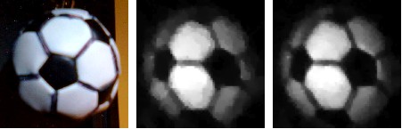
Figure 2:  Picture from a 'normal' digital camera (Left). Picture from the single-pixel camera (Middle K=800 measurements, Right K=1600, the reconstructed images have 64*64=4096 pixels).

      We performed simulations of compressive sensing, first in an optics-free case and then using the digital camera simulator ISET. Outside of the DMD which we believe was this one, none of the optical properties of the single-pixel camera were available. We took the following numbers: for the first lens f (focal length) 0.08m, F number 4; for the second lens f 0.1m, F number 4; the photodiode is a single 2.8um*2.8um pixel with integration time 0.101s and geometric efficiency 85% (which does not matter that much since there is a single pixel); we assumed monochromatic light, illuminance 90 cd/m2, and 12 bit digitization. Losses at the DMD were not simulated. For all simulations below, we took K=1024 measurements of a 64 by 64 Shepp-Logan phantom (N=4096). Note that the reconstruction will work better as N becomes bigger.

      For the optics-free simulations, we looked at different measurement matrices.We got almost perfect reconstructions with all of them.

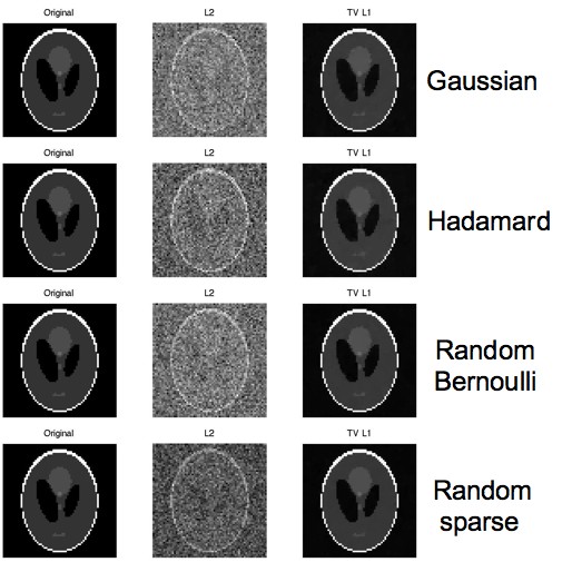
Figure 3:  Optics-free simulations with different measurement matrices. The l2 norm (least squares) performs poorly in all cases. The l1 norm minimization gives almost perfect reconstruction.

      For the optics-limited simulations, we used the Hadamard-Walsh basis as measurement basis and adapted the dynamic range accordingly. As mentioned above, alternative solutions could be found. The digitization is implemented in a simple way which does not take the effective range of the signal into account. Empirically, it has been found not to be a limiting factor (Duarte, 2008). As in the optics-free case, the l1 reconstruction outperforms by far the l2 reconstruction. However, the reconstruction is not perfect anymore, as expected.

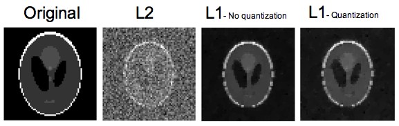
Figure 4:  Optics-limitics simulations with and without quantization. The l1 minimization reconstruction is much better than the least squares reconstruction, but the phantom is not perfectly reconstructed anymore because of the blur introduced by the two lenses.

      In (Duarte, 2008) a Daubechies-4 wavelet basis is used for the sparse reconstruction (i.e., as basis where the signal is known to be sparse). However, cscamera_test.m provided here is using the mesurement matrix directly, so we believe that the original signal was assumed to be sparse, without the need to do any transformation. We used the same assumption in our simulations. We also tried to used the Fourier basis as sparse basis (since the Shepp Logan phantom has a sparse Fourier representation) but did not get good reconstruction so far (even in the ideal case, without the optics), probably because of the parameters used and the bad conditioning of the matrices. cscamera_test.m is using a total variation minimization with quadratic constraints, whereas we used a total variation minimization with equality constraints and slightly different parameters. Our goal was not to reproduce their results (since none of the optics was known anyway), but to get an idea of the relative contribution of the reconstruction and the optics to the imperfections seen. We have provided a framework in which further, more precise simulations, could be performed.