Compressive Sensing
A signal f is said to be K-sparse if f has less than K non-zero entries.
To generalize to signals where most entries are small but not zero, a
signal is said to be compressible when it is well approximated using K terms.
Old and new paradigms
The Nyquist criteria states that a signal needs to be sampled at a rate greater than one over twice its
bandwidth. If the signal is a vector of length N, we need N samples to
reconstruct it. The sensing or measurement matrix is a N*N square
matrix. For example, below is a 1D Fourier transform matrix.
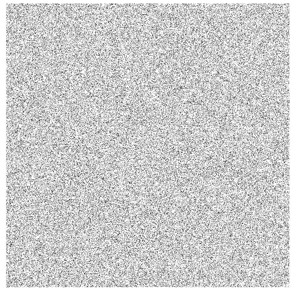
Figure 1:
1D Fourier square measurement matrix.
Compressive sensing states that if the signal of length N has a S-sparse
representation (i.e., one can find a basis in which its representation has less than S non
zero entries), then K measurements are enough, where K is greater than
C*S*log(N). C is a constant. The measurement matrix is now a K*N fat
matrix and needs to be uncorrelated with the matrix used to transform the
signal into its sparse representation. Random matrices are often used since
they will most likely be uncorrelated with any specific matrix.
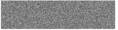
Figure 2:
Randomized Walsh - Hadamard fat measurement matrix.
Counterexample
Let us define the Fourier transform as:
If N is a square number and f the indicator function of the multiples {0,
√N, 2√N, ..., N-√N}, f is √N-sparse. F is sparse as
well, since f is its own Fourier transform. However, compressive
sensing does not apply: if we measure only a few coefficients of f, we
will likely hit only zeros and we won't be able to distinguish f from the
zero function.
For the sake of concreteness, you can run counterexample.m.
More elaborated counterexamples can be found, but the functions involved are all very structured,
as the one above. This gives us an intuition on why random is called for
help. This is also where the new paradigm of compressive sensing fundamentally parts with Nyquist.
Reconstruction
We need to solve a matrix equation of the form Cx = y where x is the signal we
are looking for, y is the measured vector and C is the measurement
matrix. Since x is of length N and y of length K with K < N, it is
underdetermined.
As an engineer, you may try to use least-squares i.e., to find the minimum l2 norm solution. Unfortunately,
doing so you are looking for the intersection of a sphere and a plane,
which will most likely not be on a coordinate axis where sparse
solutions lie.
Mathematicians have shown that the solution to
this equation is the sparsest one (Restricted Isometric Property of the
measurement matrix C). The l0 norm of a vector is defined as the number of non-zero coordinates of this vector. So, if you look for the minimum l0
solution, you will find the original signal
(Baraniuk, 2007; Candes, 2006). Unfortunately, looking for such a solution is a
combinatorial problem, which is NP-hard in general.
Looking for the minimum l1 solution is a convex optimization
problem, which can be solved numerically very efficiently (Boyd, 2004).
It has been shown that the solution found is the same as the minimum l0 solution for most
large underdetermined equations (Donoho, 2006).
Intuitively, using l1, you are looking for the intersection of a plane and a
polyhedron. You can think of the polyhedron as being "peaky", so this
time the intersection will most likely lie on an axis. Many packages can
be found which implement different algorithms performing the l1
minimization. The one I used can be found there.
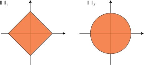
Figure 3:
Norm comparison
In a nutshell
Compressive sensing has some nice
features. First, as the number of measurements increases, the reconstruction
error decreases almost at optimal rate. Then, it is a democratic procedure:
all measurements are equally (un)important, which makes it robust, since
losing a few measurements does not matter. Furthermore, the recovery does not depend
on the acquisition: if we find a better reconstruction algorithm, we
can use it on previously acquired data. Eventually, from a technological point of
view, the complexity has been shifted from the sensor to the processing
(which software people will take as a victory).
Most papers on Compressive Sensing have been referenced in those Compressive Sensing
Resources.