Color Interpolation Using Alternating Projections

This algorithms is developed by B. K. Gunturk, Y. Altunbasak and R. M. Mersereau at the Georgia Institute of Technology [1].

Objective of Algorithm

In digital cameras that uses the Bayer Pattern filter array, the green channel is sampled at higher frequencies than the red and blue channels. Therefore, details in the green channel are better preserved than in the red and blue channels since the green channel is less likely to be aliased. Interpolation of the red and blue channels thus becomes the limiting factor in performance. In particular, color artifacts caused by aliasing in the red and blue channels are very severe at high frequency regions such as edges. The objective of this algorithm is to reduce the amount of red and blue channel aliasing by using an alternating-projection scheme that uses inter-channel correlation effectively.

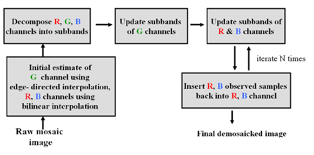
The block diagram of the algorithm is shown below, and details of the algorithm are explained later.

Detailed Explanation of the Algorithm

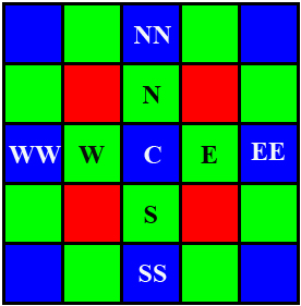
The Bayer Pattern below will serve as a reference for how positions are referenced in all the equations.

1. Initial Interpolation
Interpolate the red, green and blue channels to get initial estimate RGB values. The red and blue channels are interpolated using bilinear interpolation. The green channel is estimated using an edge- directed interpolation

2. Update Green Channel
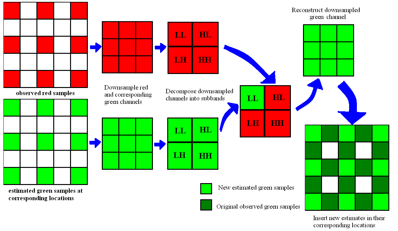
The green channel is updated by first, use the observed samples of the red channel to form a downsampled version of the red channel, and the corresponding estimated green sample values to form a downsampled version of the green channel. Then, decompose the red and green downsampled channels into their subbands, and replace the high frequency subbands (LH, HL, HH)  of the green channel with those of the red channel. After that, reconstruct the downsampled green channel, and insert the pixels in their corresponding locations in the initial green channel estimate. This procedure is then repeated to estimate the green channel with the blue channel. The figure below shows how the green channel is updated using observed red samples.

Although the example only shows 1 level of decomposition, we can do 2 levels of decomposition by further decomposing the LL subband.

3. Detailed Projection

Define as the subband of a 2D signal S  where S can be the interpolated R, G or B channels.
 the low-pass subband of S
 the horizontal detail subband of S
 the vertical detail subband of S
 the diagonal detail subband of S

Residue rk =  -  where
 Setting the threshold T, we update the detail subbands (LH, HL, HH)  of the red and blue channels using the criteria below

      where

 T is a way of controlling the amount of correlation between the channels. If the channels are uncorrelated, then T should be large. If the channels are highly correlated, then T should be close to zero. In our problem, since the channels are highly correlated, we can set T to be zero.

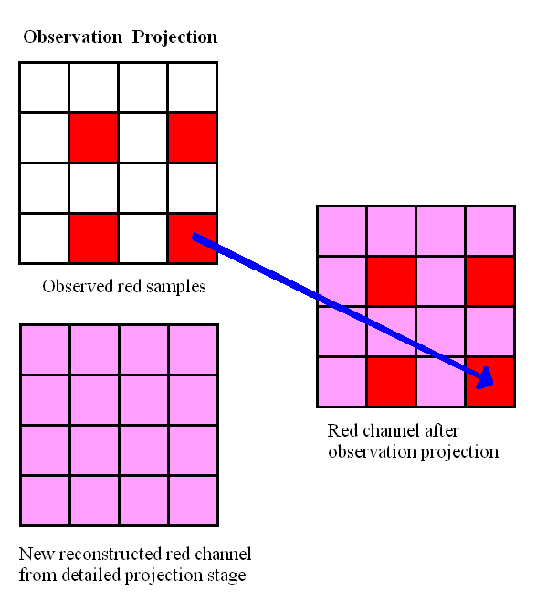
4. Observed Projection
With the new reconstructed red and blue   channels, we insert the original observed samples in these samples into their corresponding locations.
An example for observation projection of the Red channel is shown below

5. Iteration
The Detailed Projection and Observation Projection steps are iterated the number of iterations specified by the user. The demosaicked image is obtained after the iterations.