EyeLab: An Automated LED display analyzer

Methods

As mentioned, we developed three algorithms to ‘‘read’’ the digits on a 7-segment test equipment display. These algorithms were tested on two datasets. We first describe the datasets, then the algorithms, starting below.

Test Data Generation

To test the robustness of the algorithms, decoupled from noise (and other objects present) in the acquired “real data,” a series of test images were created. Utilizing the LED7 plugin for MATLAB [1], the digits 0-9 were rendered and saved as TIFF images. This plugin utilizes the fact that LED and LCD digit displays are typically of the “seven segment” variety — that is, there are seven “on or off” positions that are sufficient to convince us that something we are seeing is a particular digit. The seven segments are all visible in the representation of the number “eight,” and they are numbered in Figure 1 below:

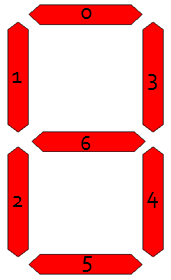
Figure 1 - Representation of seven segments used to form a digit.

With the ten digits created, the next step was to render them at various perspectives (camera angles) to simulate the possible images that could be encountered in a real laboratory setting. Figure 2 shows the simulated camera setup.

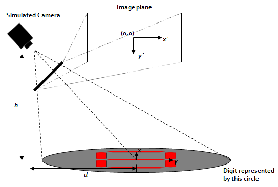
Figure 2 - Diagram showing the location of the simulated camera.

The pinhole perspective equations are used to render each digit at a variety of camera angles.

$displaystyle x' = frac{dcdot x}{y + d}, y' = h - frac{dcdot h}{y + d}$

The above equations give us new, transformed coordinates, whose “

-value” (in this case, a binary “red or white”), is equal to the the

-value at the original (x,y)

coordinates. Due to the non-linearity in the equations, the new transform coordinates are not linearly spaced. Computer images, as we know, are represented by a linear grid of pixels, thus we must interpolate our transform coordinates to a linear grid. This can be accomplished by the MATLAB griddata function. After this is done, for a particular

and

, we can create images like that shown in Figure 3. Note that we assign arbitrary dimensions to the “flat digits” — they are 0.586 units tall by 0.469 units wide.

Figure 3 - An "eight" rendered at a

of 1 and an

of 2. Original image was 0.586 by 0.469 units.

The reader will notice that so far, no attempt has been made to rotate the perspective — the digits have been looked at either dead-on or from one of the sides. In a real setting, however, there is no guarantee that the camera’s view will not be rotated. We could, for example, be looking at the digit from “down and to the left” which would result in a rotation. To account for this, the “original” flat digit was rotated and the perspective was recomputed. This resulted in additional test images, such as that shown in Figure 4.

Figure 4 - An "eight," rotated 40 degrees, and rendered at a

of 1 and an

of 2.

We now have an understanding of the parameters that are adjustable to create digit images, namely rotation angle theta , distance , and height . One thousand images were created, 100 per digit, with a fixed of 2, a spanning in unit increments from 1 to 10, and theta spanning in ten degree increments from zero degrees to ninety degrees.

Real Data Acquisition

Video Capture

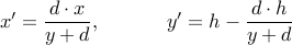
A FujiFilm Z5 point-and-shoot digital camera was used to capture all video. Video was captured at 30 frames per second, at a resolution of 640 times 480 pixels, and was compressed on-camera using MotionJPEG compression.

Figure 5 - FujiFilm Z5 camera used to capture video.

Test Equipment

A Tektronix DM511 digital multimeter was connected to a function generator. A 0.1 Hz, no-offset, 100 mVpp sine wave was fed into the voltage read terminals of the multimeter.

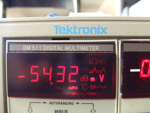
Figure 6 - Frame capture (scaled down) of video of Tektronix DM511 multimeter.

The digits of the multimeter were recorded by the camera for approximately 40 seconds. Note that all digit ID algorithms ignored the negative sign, thus rectifying the input signal. Figure 7 shows us both the actual input to, and “expected output” from our algorithms.


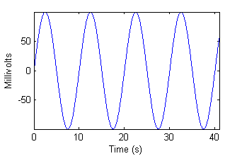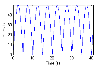Figure 7a - Input from function generator.	Figure 7b - "Ideal" algorithm output.

Algorithms

Generic Pre-processing

Before any algorithm is applied, some preprocessing steps are taken to ensure the input image is as “clean” as possible. The steps are as follows. While many of the steps require user input on a sample frame of video chosen at random from the input video file, the same preprocessing is applied to all video frames.

The user is asked to draw a bounding box around the digits of interest. The assumption here is that the camera or the test equipment is not moving at all throughout the duration of the experiment.
The user is asked how many digits there are. The image’s columns are then split into equally sized chunks from left to right, where is the number the user entered.
The user is asked to indicate which “chunk” contains a decimal point, and whether or not the decimal occurs after or before the digit in that chunk.
The user is then asked to draw a bounding box around the decimal point. The software automatically deletes the decimal point from all frames.
The user is then shown the red, green, and blue channels of the image, and asked which one most predominantly captures the digits. The other channels are eliminated.
The resulting one-channel image is binarized. To do this, first the image is scaled to a zero to one range. Next, all values above 0.8 are assigned to 1, and all remaining values are assigned to zero.
The user is then asked to choose one of three algorithms to process the data–they are explained below in the subsequent three sections.

“Smart-strokes”

The underlying principle behind the “Smart-strokes” algorithm is simple: there are only seven possible segments, and since we know where they should be, it should be relatively straightforward to see which ones are illuminated. To facilitate different “fonts” from different test equipment, seven “rather large” overlapping regions are chosen to represent the seven segments. These are indicated by the shaded regions in Figure 8. Note that the regions are defined in terms of relative height and width, making this a scale invariant method of digit identification.

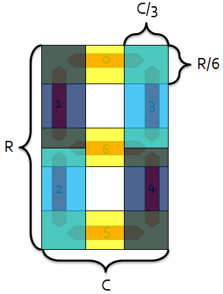
Figure 8 - Overlapping shaded "segment regions" for Smart-strokes algorithm.

We can define a particular digit by a vector in 7-space, where each element of the vector (indexed according to Figure 8) corresponds to whether or not that segment is illuminated. For example, the digit four would be represented by the following vector:

displaystyle v_4 = [0, 1, 0, 1, 1, 0, 1]

This is shown graphically in Figure 9:

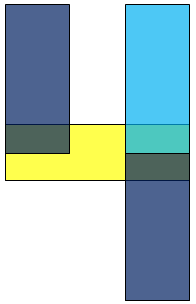
Figure 9 - "Smart-strokes" shaded regions for the digit "four."

Having created our vectors, we can now explain the algorithm. It consists of the following steps:

Each pre-processed digit is put into a bounding box algorithm to find the tightest bounding box for the digit.
If the bounding box is more than 2.5 times as tall as it is wide, the digit is automatically classified as a “one.”
The image is cropped to the bounding box, and each of the seven “Smart-strokes” segments are pulled from the cropped image.
For each segment, if more than 40% of the segment is illuminated, the segment is considered “on.”
A vector , representing the illumination pattern, is assembled in the same way that we assembled the vectors above.
The digit is classified using a simple nearest-neighbor classifier. Our best guess is determined by the following:

argmin $_{iin{0,9}}($ norm [q-v_i])

This process is repeated for all the digits on a particular image frame, then repeated for every frame, until all frames have been processed. For each digit, the “Smart-strokes” algorithm has O(1) complexity, making it run quite fast (see results). For digits, we have O(M) complexity.

DCT Cross-correlation

Creating Matched Filterbank

This algorithm is essentially a bank of matched filters for each digit. There are two challenges: first, creating the matched filters themselves with no a priori knowledge of the “font” of the particular test equipment, and second, making the matched filters invariant to scale, rotation, and translation.

For the first challenge, an attempt was made to use the test images generated in MATLAB to create the matched filters for the real data. With a human, this would work — if we see the computer generated “four,” we would be able to pick a “four” from a similar 7-segment display without problem. Unfortunately, after much trial and error, this method did not work. Thus, I decided to implement a brief “training period” before the algorithm runs. The “training period” is as follows:

The user is shown and asked to identify a series of digits chosen at random from the data.
More digits are shown to the user until the user has identified two of each digit. This is kept track of automatically — as soon as the user has found two of each digit, the training ends. Note that this means that many more than two of some of the digits will likely be found, as the digits are randomly chosen.

With some digits identified by the user, only the second challenge — transformation invariance — remains. It is surmounted by the following:

The pre-processed, now identified digit images are fed into a bounding box algorithm, which finds the tightest bounding box for the displayed digit.
Each image is cropped to this bounding box.
Each cropped image is resampled to a fixed 70 row 40 col. pixel window. This often involves downsampling, but in the cases of low resolution images, upsampling with linear interpolation (via MATLAB’s interp2) is used. This resampling takes care of scale invariance.
The resampled image is normalized to zero mean and unity standard deviation.
The Discrete Cosine Transform (DCT) of each cropped image is created and stored, with some identification as to which digit this DCT represents. Since the magnitude of the DCT is not affected by translation, this takes care of translation invariance. Note that the bounding box also helps with translation invariance, but in the event that the binarization was noisy and the bounding box was not “perfect,” the DCT’s translation invariance comes to the rescue.
Each DCT is stored as a matched filter for the digit it represents! We end up with, at the minimum, two matched filters per digit.

Figure 10 shows an example of some examples of matched filters:

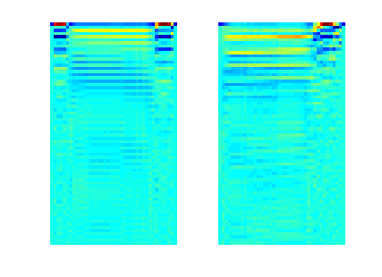
(left) Figure 10 - DCT matched filter for digit "zero" (right) DCT matched filter for digit "three."

Note that I have not yet accounted for rotation invariance. This is tricky — making an image be “upright,” is complicated, especially by the fact that many 7-segment digits are actually somewhat slanted (not rotated) to begin with. Correcting for this will be a subject of future work, but it should be noted that since the identified digits used to create the matched filters come from the actual data, this problem is mitigated.

Identifying Unknown Digits

With at least two matched filters for every digit, the remainder of the digit identification is very straightforward.

Each incoming “unknown” digit is cropped, resampled, and its DCT is taken, identically to the processing of “known” digits explained above.
A point by point multiplication is taken between each digit and all the matched filters. This is equivalent to the 2D cross correlation evaluated at the origin, which is equivalent to the dot product of the image with the matched filter if they were considered to be vectors.
For each digit possibility (0-9) the average of these cross correlations is taken. For example, if we had four identified digit “one” matched filters, then we would perform the above step four times, then divide by four (then, of course, repeat for the rest of the digit possibilities). Remember again that the minimum number of matched filters per digit is two, but we could have more depending on which order the digits were presented to the user for identification during the training phase.
We now have a “likelihood score” for each digit: the “average” dot product between the unknown digit and the pre-identified digits zero through nine. Just as before, this is a type of nearest-neighbor classifier — the “closest in norm” (maximum dot product) matched filter identifies the unknown digit.
The above process is repeated for all digits in all frames (including the already identified digits). For each digit, this algorithm is of efficiency — the point by point multiplication requires looping over every pixel in the image. This is still quite fast. If we were considering additional cross-correlation points than that evaluated at the origin, the algorithmic complexity would approach ! Remember, of course, that when considering digits, the complexity is still .

Automated Feature Extraction/Neural Network Classifier

This method utilizes an automatic feature extractor to extract six features from each digit, then feeds these into a neural network for classification.

Feature Extraction

The preprocessed image is fed into MATLAB’s regionprops command to extract six features. These features were chosen because they were (intuitively) the most “relatively” scale, transformation, and rotation invariant features present [2]. The features are described below:

Centroid — The “center of mass” of the image. Since it is binarized, we can represent the image by a series of points (2-vectors) . The centroid, , is then:
$displaystyle vec{C} = frac{sum_i p_i}{N}$ Note that this, in the implementation, is treated as two features because the and coordinates of the centroid both count as a feature.
Perimeter — Best described by MATLAB’s documentation [3], the perimeter is “the distance around the boundary of each contiguous region in the image.” For our purposes, each digit, in its entirety, is treated as one contiguous region.
Major Axis Length — After an ellipse is fitted to the data, this feature is the length of its major axis. Note that this is rotation invariant.
Minor Axis Length — Similar to the above, but the minor axis.
Eccentricity — The eccentricity, another parameter of an ellipse, is the ratio of the distance between the foci to the length of the major axis. If and are the semi-major and semi-minor axes, the eccentricity can be found by the following formula:
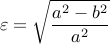
$displaystyle varepsilon = sqrt{frac{a^2-b^2}{a^2}}$
Orientation — The angular orientation of the major axis of the ellipse. This is rotation variant, but was thrown in “for good measure.” If the neural network “works,” it will ignore this if necessary.

Classification

The features described above were fed into a neural network classifier, created using MATLAB’s neural networks toolbox. The classifier is diagrammed in Figure 11.

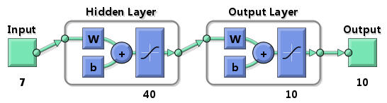
Figure 11 - Neural Network Classifier

There are seven input neurons corresponding to the seven features listed above (six plus an extra for the two centroid coordinates). Next, there is a hidden layer with 40 neurons. Finally, there are ten output neurons, each corresponding to a digit. The desired response vector corresponding to a particular digit is a 10-vector with all zeroes except a one at the index of the digit. For example, the desired response for the digit “four” is:

displaystyle d_4 = [0, 0, 0, 0, 1, 0, 0, 0, 0, 0]

The actual training of the network is described in the following section.

Experimental Setup

Two “experiment groups” were run. The first tested the abilities of the neural network classifier, and the second tested the other algorithms. All algorithms were run with three resolutions of data — the original, a 2X downsampled in both dimensions, and a 4X downsampled version.

Neural Network

Since we didn’t have identification information for the “real data,” only the simulated data could be used. The one thousand test images were randomly subdivided into two categories: training and testing. 30% of the data (300 digits) was used to train the classifier, and the remaining 70% (700 digits) was used as “raw input” to see how well the network could identify digits that were not training patterns. The network was trained with the scaled conjugate gradient backpropagation algorithm [4].

Smart-strokes and Cross Correlation with Test Data

The one thousand test images were arranged into an AVI file, such that the first hundred frames were different “views” of the digit zero, the second hundred of the digit one, etc. This AVI file was run through the three algorithms, and the mean square error (MSE) of digit identification was computed. This was possible because we “knew” what each digit should be (we couldn’t say this for certain with the real data without first manually identifying each digit — a time consuming task!). Note that for the test data, the “training” step in the Cross-correlation method was not interactive — that is, random digits were still chosen to be identified for creating the matched filters, but they were identified automatically.

Smart-strokes and Cross Correlation with Real Data

The AVI file was loaded from the camera on to the computer, then directly into each algorithm. Again, I could not run this data with the Neural Network algorithm, because the amount of needed training data was too great, and would have taken too much time to manually create. The performance of the remaining two algorithms was evaluated qualitatively by comparing the output to Figure 7b. Specific “error frames” were picked from the video upon inspection of Figure 7b, and were analyzed to determine the cause of the errors.

Metrics

Mean-Squared Error

To determine the accuracy of the algorithms when using the test data, the mean-squared error was computed. For clarity, we define what me mean by “squared error.” If, for example, we are looking at a “five,” but the algorithm thinks it’s a “seven,” the squared error is (5 - 7)^2 = 4 . The mean of these squared errors determines the mean-squared error. Note that we have chosen MSE instead of more “typical” classifier statistics (sensitivity, specificity, etc.) because, in the end, we’re trying to reconstruct a time trace. With time traces, we care if something is “off by a little” or “off by a lot” — this information is captured by MSE but not by sensitivity and specificity. MSE, as we’ve defined it, has an intuitive meaning: if the algorithm has an MSE of , this means that we can be confident of the guessed digit with (roughly) a standard deviation of sqrt{E} .

Run Time

The runtime was recorded to demonstrate the feasibility of implementation of the algorithms. All experiments were run on my Lenovo T61p Laptop, which has a 2.20 GHz Core 2 Duo CPU, 4.00 GB ram, and is running 64-bit Vista.