EyeLab: An Automated LED display analyzer

Conclusions

Quantitative Examination

Before examining the results more closely, one should note that the “Test Data” and the “Real Data” are not “testing” exactly the same thing. The “Test Data” shows digits from different camera angles, while the “Real Data” shows digits from the same angle. Because the “Test Data” is computer rendered, if the camera angle were fixed, the image will look exactly the same at each frame of rendered video. This is not true of the “Real Data,” where fluctuations in the light level of each segment of each digit of the test equipment (sometimes exacerbated by the image binarization algorithm) can lead to one digit looking different in each frame of video. This is shown below in Figure 18.

Figure 18 - Three examples of "three" pulled from the "Real Data."

Intuitively, and as we can see in the above figure, changes in light level do not cause as much variability as changes in camera angle. Thus, one would expect the MSE in identifying the “Test Data” to be an upper bound to the error observed in a “real world” setting.

This is confirmed upon closer examination of the confusion diagrams (Figures 12 and 13). One will notice that with the exception of “eight” with cross-correlation, all of the digit misidentifications occur near the ‘‘beginning’’ of each of the one hundred ‘‘runs’’ of a particular digit. Recall that when the test data was created, was spanned from 1 to 10. The ‘‘earlier runs’’ of each digit, then, correspond to digits that were ‘‘closer to the camera’’ thus more distorted! We’ve already seen an example of this in Figure 4. From this, we come to two important conclusions. First, we confirm that the ‘‘Test Data’’ is an upper-bound for MSE, because rarely in the real world will we have cameras that are extremely close to the digits. Not only would this be too close to see the neighboring digits, but most camera optics can’t focus very close without a special lens. Second, we confirm visually that the MSE of the cross-correlation method is in fact lower than “Smart-strokes.”

The confusion diagrams also provide some insight as to ‘‘why’’ certain digits are identified incorrectly. With “Smart-strokes,” many digits are incorrectly identified as a seven. This intuitively makes sense. Seven has three illuminated segments: the top segment and the two right segments. Many digits also have the top and the bottom-right segment illuminated. If changing the camera angle were to make only some segments of each digit appear to not be illuminated, there is a greater chance that these two will remain illuminated because they are more likely to be illuminated in the first place. Note, also, that many ‘‘eights’’ are mis-identified as a smattering of other digits. This also makes sense — ‘‘eight’’ illuminates all the segments, thus turning one or two off at random can readily turn it into other digits. This also suggests why, in the cross-correlation method, that eight is the most readily misidentified digit. With its abundance of illumination, it looks a lot like six and zero. It’s no surprise that the DCTs are similar and thus it is most commonly misidentified as these other digits.

With all of this said, the Neural Network method performs better by an order of magnitude MSE and run-time than the other algorithms. This is to suggest that, despite my best efforts, it is more robust to changes in camera angle (i.e. translation, rotation, skewing, scale, etc.) than the other methods. Remember, however, that it uses significantly more “training” images (300!) than the cross-correlation method (which only uses around 2-4 of each digit) or the Smart-strokes method (which needs no training!). Since this cannot be used (easily) with “Real Data,” we conclude that the “best” method to use is the cross-correlation method, which offers great performance at reasonable compute times. Finally, in terms of both performance and run-time, all three algorithms can agree on one thing: downsampling leads to decreased performance and increased runtime. Interestingly, the performance is not that much worse at 4x downsampling, suggesting that these algorithms could be implemented with a webcam in real time!

Qualitative Observations

Figures 12-15 look very similar to our “expected” waveform in Figure 7b, except for two main differences: quantization artifacts and random “spikes” throughout the waveform. The quantization artifacts are actually due to the sampling rate of the multimeter (about 2 Hz). Our video camera, at 30 FPS, grossly oversamples the multimeter! The “spiking” artifacts, at first, appear to be errors in digit identification. While this is true in some of the cases, in many cases, this is in fact an error from the multimeter! Take the first major “spike” around five seconds. Both algorithms in fact correctly identify this, shown in Figure 19, as 98.08 millivolts.

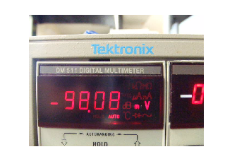
Figure 19 - Mistake in multimeter output.

That said, the two methods don’t always have the same “spikes” so we know that there are definitely some errors being made. Specific to the “Smart-strokes” algorithm, we notice a fair bit of oscillation around 30 millivolts–sometimes the “three” is being identified as a “four,” and vice versa. This gets worse as the spatial sampling rate is reduced. Interestingly, cross-correlation appears to work better as sampling rate is reduced (contradicting the “Test Data” results) — Figure 15 looks very clean. Somehow, the “spiking” has been corrected for!

Since 30 FPS is too much for monitoring most test equipment, we can use the advantage of oversampling to create a robust moving average of the data to “smooth out” the quantization and the spikes. Alternatively, the sampling rate could be reduced, or, we could take “bursts” of 30 FPS at predefined intervals. For example, if we want to read a voltage once every hour, we could automatically turn on the camera for ten seconds each hour and take a fairly long average for each hour’s single time point.

Final Words

Thus, we have demonstrated a system whereby test equipment can be monitored using an ordinary digital camera. With a minimum amount of training, the Cross-correlation algorithm can be used to identify the digits very rapidly and with high accuracy. If more speed is desired at the cost of accuracy, the “Smart-strokes” algorithm can be used. If we have more time to manually identify digits coming from the video, a robust feature extractor and Neural Network classifier can be used to read the digits with high accuracy. All of the methods are computationally inexpensive and, since they are robust to a reduced spatial sampling rate, could likely be implemented in real time.