Results

On-Axis Light Results

The first optimization we ran was for a standard wire arrangement. Only one metal layer was taken into account. Light was incident at an angle of 0 degrees, the metal wires were separated by 1.9 μm and were not shifted along the x-direction (image on right). No unusual or counterintuitive results were expected. Initially, wire shift along the x-axis was varied between values of –1.65 and 1.65 μm, and cost was calculated at a step of 0.1 μm (below). As expected, the optimal shift was 0 μm; an expected result since light was incident on-axis. Next, separation (aperture size) was varied from 0.5 to 5 μm, and cost was calculated at a step of 0.1 μm (also below). Here, the local minimum was not calculated, but using visual estimation, the point of diminishing returns was found to be approximately 1.5 μm. In other words, increasing the separation between the wires by more than 1.5 μm did not significantly improve the overall power ratio. 

Figure 1: Pixel diagram.

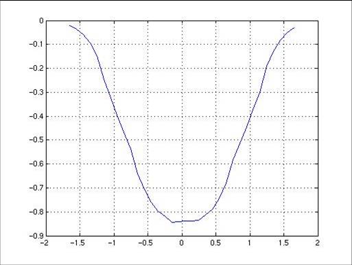
Figure 2 : Cost vs. Shift (above).

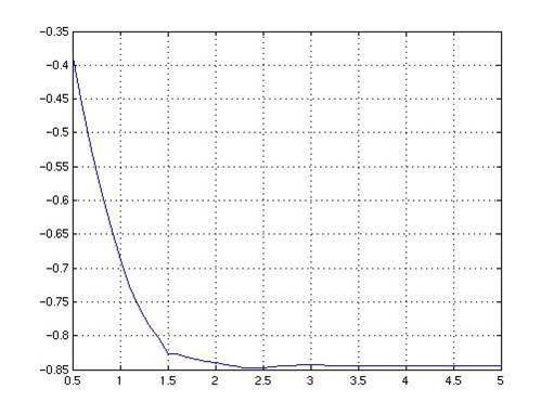
Figure 3 : Cost vs. Aperture size (above).

Off-Axis Light

Next we explored the off-axis case (incident light at 10 degrees) to see what happens to a pixel to which light enters at an angle.  We expected that counter-intuitive results would be more likely in an off-axis pixel when the light is not simply directed straight down.  First, to get a sense of the cost function to be minimized, we considered one metal layer at a time by widening the aperture of the other two layers to be larger than the pixel width.  Taking each metal layer separately we plotted cost (the negative of the overall power ratio) versus aperture width.  These results are not shown since they are generally the same as the on-axis case (see Figure 3), namely wider aperture size was always better.  A point of diminishing returns was reached, however, around 2.5 μm. 

Next, cost versus shift was determined for each metal layer (Figure 4, below).  Here it is clear that an optimum horizontal position could be determined for each metal layer, and that the local minimum of the cost function would also be the global minimum.  In addition, two trends stand out across the three metal layers.  First, the further down the pixel, the larger the optimal shift, as illustrated by the rightward shift of the curves across Figure 4.  This result was expected; in order for light entering at an angle to pass freely through the apertures, each successive aperture needs to be shifted more. 

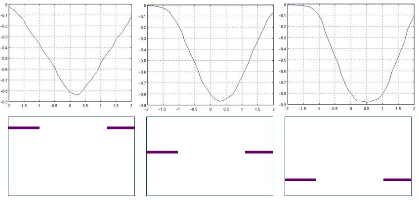
Figure 4 : Cost vs Shift, in microns (um) for each metal layer (A-C) independently. Schematic of pixel below; corresponding graph of cost vs shift above.  Cost is defined as the negative of the Overall Power Ratio.  Line and number indicate result of fminsearch.

The second trend is in the shape of the curves.  For the topmost metal layer, the cost function is rather steep around the minimum, whereas for the bottom layer there is a substantial flat portion around the minimum.  This difference corresponds to the leeway, or give, in the optimal position.  For the topmost layer, any shift away from the optimal one will result in a decrease in power (increase in cost).  On the other hand, small changes to the bottom layer’s position have less of an effect.  This is intuitive, since light in the pixel has already been focused by the microlens.  Thus, the light beam will be narrower closer to the bottom than at the top, providing the bottom aperture with more leeway than the top.

Optimization Results

Having manually examined the cost functions we next turned to the MATLAB optimization function fminsearch to find the optimal shift for each metal layer.  Utilizing the optimization does not generate a figure, however it provides an exact number and does so fairly quickly.  Creating each graph in Figure 4 took 59 seconds, whereas each optimization took 52 seconds.  While this difference is not so pronounced at this level of complexity, as the complexity of the problem to be optimized increases we expect the gap to widen significantly.  The results of fminsearch for each metal layer independently are also shown in Figure 4 and (as expected) correspond correctly to the minima of each function.  Interestingly, though the metal layers are evenly spaced in the oxide, the optimal shifts are not evenly spaced as might be expected.

Once each layer was optimized independently, we re-optimized each metal layer taking into account the presence of the other two.  Instead of widening two of the apertures to remove them from the pixel, all the metal layers were set to their previously calculated optimal shifts, and one metal layer at a time was optimized by fminsearch under the new configuration.  This yielded a new and potentially improved set of optimum shifts for the wires as shown in Table 1.  Intriguingly, the shifts are even less linear than before, indicating that the metal may be altering the path of the light from its straight line between microlens and pixel floor.

Finally, we wanted to know how our two optimizations (one with one metal layer at a time, the other accounting for the presence of the other two layers) compared to one another as well as to reference pixels for incident light at 10 degrees.  These summary results are shown in Table 2.  The first reference pixel is a pixel with three metal layers centered at zero (un-shifted).  The second reference pixel is the empty pixel, a pixel with no metal at all.  It is clear that the un-shifted pixel is the worst case scenario.  Even the initial optimization is an improvement over the un-shifted pixel, both in terms of overall power and in terms of collected power.  In addition, the second optimization is a clear improvement over the first by both metrics.  Thus the more accurate pixel simulation led to an optimization that yielded better results.

Perhaps most interesting, however, is the comparison between the best optimization and the empty pixel.  Initially we predicted that any metal between the microlens and the photodiode would only interfere with the light and thus decrease the overall power.  Surprisingly, the second optimization barely alters the overall power ratio compared to the empty pixel, while at the same time better focusing the light, as shown by the improved collected power ratio.  The improvement in the focus of the light serves to minimize the potential for crosstalk between pixels, a major concern for off-axis light.  Overall, these results indicate that shifting the metal based on the second optimization leads to a pixel configuration that rivals and may even improve upon the trivial solution of no wires at all. 

Table 1 (above): Optimized position of each metal layer; comparison between two optimizations as described in text.

Table 2 (above): Power ratios for both optimizations and two reference pixels (unshifted and empty).