PART 3. Simulating the comparison of the theoretical camera’s response versus the spectrophotometer measurement response.

Now that we have our data measured by the spectrophotometer “compressed” using linear model, and our camera data “expanded” using the method described in PART 2, we can compare the two results after doing some mathematical formulations.

Our coefficients from the linear model compression of the spectrophotometer measurement are formed in a [5xN] matrix where each column represents one set of skin radiance data expressed in 5 basis weights.

On the other end, we have a [9xN] matrix from our camera where each column represents one set of skin radiance data, captured by the camera, in 9 different values (3 values from the camera under normal lighting condition, and 6 values from the camera under two different filters used in addition to the same lighting condition). Therefore, since we ought to compare the [5xN] matrix from the linear model with the [9xN] matrix from the camera result, we need to do some mathematical formulation. The following is the explanation of some parts of the code provided in this website (ProjectCode.m)

The following mathematical formulation is to approximate N surface radiance with 61-wavelength precision points generated by spectrophotometer measurements. We used 5 bases numbers. The camera has 9 channels.

From the linear model’s end we have the following variables:

• radiance as the radiance measured by the spectrophotometer
• sBasis as the default basis functions that we got from linear model computation
• coef is the set of coefficients that represent the real radiance

Since:

radiance = sBasis * coef %[61xN] = [61x5][5xN]

We can approximate coef as:

coef = pinv(sBasis) * radiance %[5xN] = [5x61][61xN]

To compare with the camera’s response, we need to add extra variables:

• cameraR is the camera’s response
• sensor is the camera’s RGB values for conditions without filter, with first filter, and with second filter
• estCoef is the camera’s estimated set of coefficients that tells us how camera captures the scene radiance

We know that camera response is:

cameraR = sensor’ * radiance %[9xN] = [9x61][61xN]

Therefore we can approximate camera response as:

cameraR ≈ sensor’ * sBasis * coef %[9xN] = [9x61][61x5][5xN]

estCoef can then be formulated as:

estCoef = pinv(sensor’ * sBasis) * cameraR %[5xN] = [5x9][9xN]

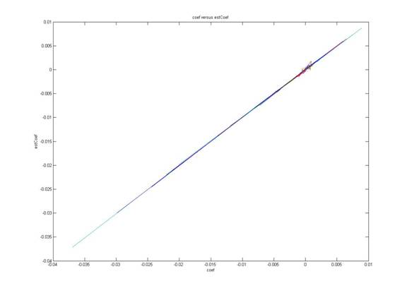
We now have two [5xN] matrices from the linear model and from the camera prediction. We can compare these two values. Figure 3.1 shows the plot of coef against estCoef. If the two values are close to each other, than we expect to see straight diagonal lines on the plot. However, we see some glitches around 0-point in the plot, which means there are slight discrepancies around that value.

Figure 3.1 Comparison of linear model coefficients (coef) and Nikon D70 predicted coefficients (estCoef).  

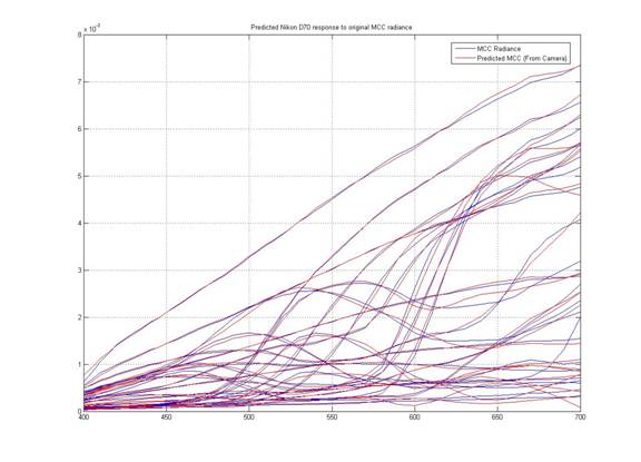
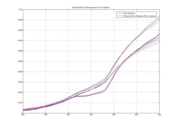
Since we are interested in knowing how well the camera captures the radiance, a more meaningful way of looking at the result of this calculation is by reconstructing the radiance data using estCoef (from the camera) and compare them with the original data.

cameraPredictedMCC = sBasis * estCoef %[61xN] = [61x5][5xN]

Figure 3.2 shows the comparison of measured Macbeth Color Checker radiance with the radiance captured by Nikon D70. Figure 3.3 shows similar figures of measured skin radiance. As we can see from these figures, Nikon D70 does a good job at both predicting the Macbeth Color Checker radiance and measured skin radiance.

Figure 3.2 Comparison of Nikon D70’s response to MCC radiance

Figure 3.3 Comparison of Nikon D70’s response to skin radiance