Part 1: The Linear Model

We have ways of capturing a lot of wavelength data, about a hundred points per pixel, using instruments such as a spectrophotometer, which will be discussed in this section. A spectrophotometer, however, does not have very high resolution. We also have ways of capturing high-resolution data using digital cameras, but cameras contain three points per pixel, which is not nearly as much as the spectrophotometer.

There is a tradeoff between the two: it would be unreasonably expensive to have a high resolution camera with as many data points per pixel as a spectrophotometer. We can, however, take advantage of linear models to retain most of the image data with more points per pixel in a camera, but far less points per pixel than in a spectrophotometer.

1.1 The Spectrophotometer

A spectrophotometer measures the spectral radiances over a surface. When light of any given spectral power distribution falls on a surface, the surface radiates back some of the light at a different spectral distribution over the same wavelengths. This spectral distribution, or surface radiance, is essentially what the spectrophotometer measures.

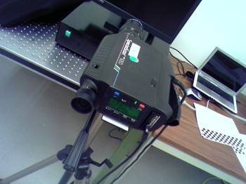
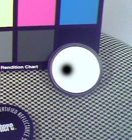
Below are two images about the spectrophotometer. Figure 1.1(a) shows a photo of the spectrophotometer, which we operate using an eyepiece and lens. Figure 1.1(b) simulates what we would see when looking at any scene through the spectrophotometer. The black spot is the area over which the spectrophotometer calculates the surface radiance.

Figure 1.1 (a). Photograph of a Spectrophotometer

Figure 1.1(b). Simulated Spectrophotometer Scene

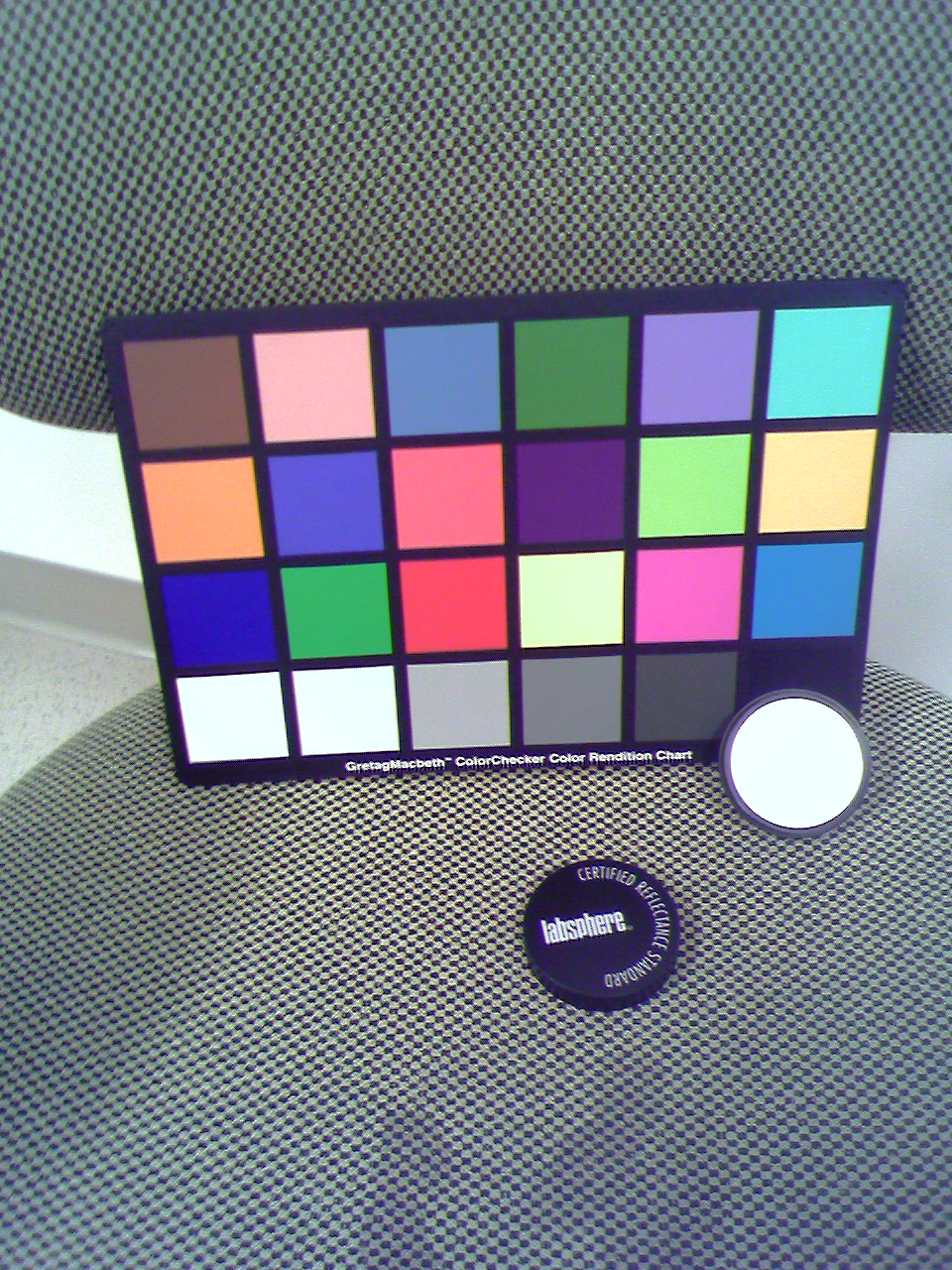
The spectrophotometer was set to measure the surface radiance at 101 different wavelengths at each surface. We measured the surface radiances of a white surface, and the Macbeth color checker, which is a standard color chart of 24 different colors

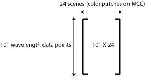
Each of the other 24 surfaces in the Macbeth color checker (shown below in Figure 1.2) produced an analogous set of data. The color signal from 24 surfaces, each with 101 data points, produced a 101 by 24 matrix.

 

Figure 1.2 (a). Macbeth Color Checker (MCC)

 

Figure 1.2 (b). Color Signal (Radiance) Matrix for the MCC Using the Spectrophotometer

1.2 Spectrophotometer vs. Camera

As we said above, the spectrophotometer produces 101 data points per surface with low resolution. A modern digital camera, on the other hand, has much higher resolution—in the simulated spectrophotometer above, the black spot takes up many pixels.

However, there are only three color channels in the digital camera: the Red, Green, and Blue (RGB) channels. The human visual system also contains three (relatively independent) color channels: the L, M, and S cones. Because of this, when the camera images are seen by humans, some of the visual data from the actual image may be lost. More color channels would help.

Obviously, it is impractical to use 101 points per pixel, as the spectrophotometer does. But can we do better than only three channels, like the camera? The answer is yes—using linear approximation.

1.3 Linear Approximation

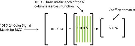
In linear algebra terms, the RGB channels create a representation of the image data using three basis functions. We want to use more than three channels; and we have 101-point data for a standard color chart which represents the entire visual spectrum relatively accurately. The equation below in Figure 1.3 shows an example of a reduction into 6 basis functions.

 

Figure 1.3: Six-Basis Representation of MCC Data

Using what we measured (or what has been previously measured) from the Macbeth color checker and from the spectrophotometer, we can derive basis functions that approximate the image, and we can choose the number of basis functions. According to [2], 5 to 6 basis functions are optimal; we’ll derive the functions and verify this.

1.4 Singular Value Decomposition (SVD)

We will derive the basis functions using a mathematical technique called Singular Value Decomposition (SVD). The general idea of SVD is to take the data from the sample surfaces (in our case, the Macbeth color checker; 24 samples, each with 101 data points) and decompose it into a set of bases in order of importance and a set of weight values that describes the relative importance of each basis. This is exactly what we want, since all we have to do is pick the first N bases and N weight values in order to have a basis of size N. With the spectrophotometer samples, we can have up to 101 bases.

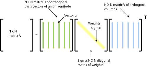
The equation below shows the SVD of a matrix A.

The columns of U form an orthogonal basis, with vectors ordered from greatest to least in their importance. The diagonal entries in Sigma are the weights. We use the basis matrix V to help calculate the SVD, but it is of little value for the results we want. To make SVD easier to visualize, the matrix form of the SVD is also shown below in Figure 1.4.

 

Figure 1.4: SVD matrices

To compute the SVD of any matrix A, assume that A has the SVD form shown above and multiply A by its transpose. The product of the SVD with its transpose becomes

This is essentially the eigenvalue decomposition of A TA. We can exploit this fact to calculate V and Sigma. V contains the eigenvectors of A TA, and the eigenvalues of A TA are the squares of the diagonal entries of Sigma. We can now solve a matrix equation for each column of U using the formula

.

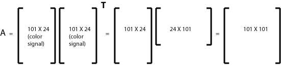
For our purposes, A is the symmetric matrix formed by taking the samples and multiplying them with their transpose (in other words, A = [samples][samples] T), as shown in Figure 1.5. Also, note that in Matlab, the SVD can be calculated using the command [U,S,V] = svd(A))

Figure 1.5: Matrix Formation of A

As stated before, we can choose the first N columns of U and the first N diagonal entries to get a basis of size N.

1.5 Determining the Basis Size

We want to generate a set of bases that predict the spectrophotometer data relatively accurately. To find this, we can start with a minimum number of bases, and gradually increase the number of bases until the mean square error between the predicted and measured reaches a satisfactorily low value.

The graph below shows the mean square error between the predicted and theoretical radiances of the Macbeth color checker as a function of the number of bases. One basis produces a relatively large error, and the error decreases sharply as the number of bases increases to two, three and four. After adding more bases to a set of four, however, the error slope starts to decrease. We start getting only marginal improvement with five and six bases; it doesn’t make sense to keep increasing the number of bases; five or six bases appears optimal. This seems to confirm the results presented in [2].

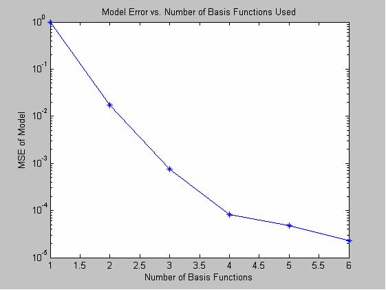
Figure 1.6: Mean Square Error Between Estimated and Measured Radiance Spectra vs. Number of Basis Functions

1.6 Predicting the Spectral Radiances of Surfaces

Now that we have determined an optimal number of bases, we can use the basis functions to predict the spectral radiances of the surfaces in the Macbeth color checker. The optimal values are again five or six bases; we use six bases in the following calculations. Recall that the Macbeth color checker can be reduced to a function of 6 basis vectors, as shown earlier in Figure 1.3.

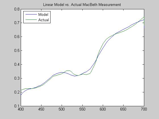
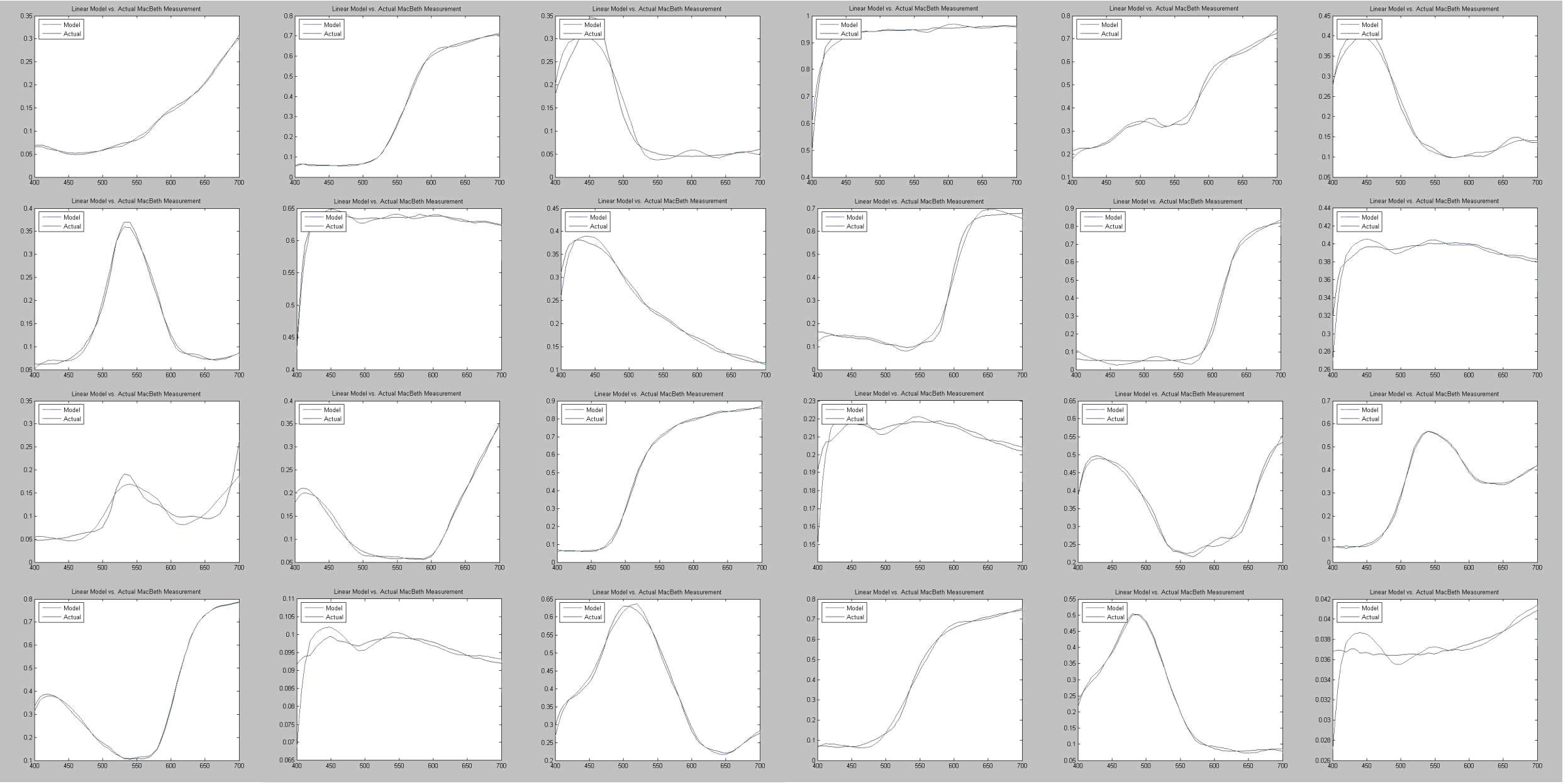
We can use a least-squares approximation to find the 6 by 24 coefficient matrix, since the spectrophotometer data is given and the bases are already determined. Using these values, we can plot the approximate curves for each of the 24 surfaces in the Macbeth Color Checker. Figure 1.7 shows one enlarged plot of approximate and actual surface radiances of one surface and an array of smaller plots of each of the 24 color surfaces in the Macbeth color checker. As shown, the linear model and the measured data seem to be very close with six basis functions. This indicates that the linear model developed in this project is a good predictor of the Macbeth color chart. Since the Macbeth chart is used as a standard for many applications, the linear model is also pretty good at estimating radiances in other surfaces, such as in camera images, as will be shown in the next part.

Figure 1.7(a): Estimated and Measured Radiance Plots for One Surface in MCC

 

Figure 1.7(b): Estimated and Measured Radiance Plots for all MCC surfaces (click here for real size picture).