Fig. 2-1. CFA pattern sampling and its frequency domain representation
|
Evaluation of Noise Characteristics in Image Pipeline |
| Annabel Huo, Hyung Suk Kim, Sung Hee Park March 21, 2009 Psych 221 : Applied Vision and Image Systems |
| | Introduction | Methods | Results | Conclusions | References | Appendix | |
| | Basic Model | Demosaic | Denoise | Pipeline | Joint | Comparison | |
| Basic Model Analysis | Top |
| CFA Pattern and Sampling |
|
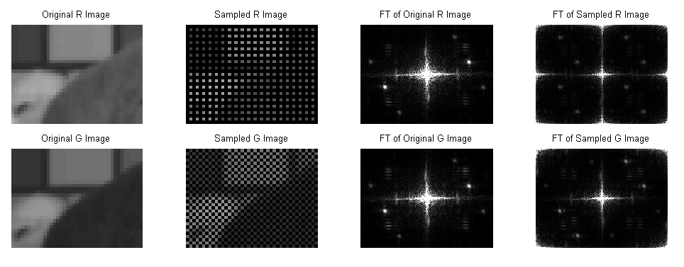
Fig. 2-1. CFA pattern sampling and its frequency domain representation |
|
We use color filter array to get RGB images from one image sensor because an image sensor can capture only a single value per pixel. However, a captured image does not contain all RGB data in every pixel, which requires demosaicing process to get desired RGB color image. Applying color filter array can be understood as sampling operation applied to pixel values for each channel with different sampling pattern. In other words, a captured RAW format image is the combination of sampled images for each R, G, B channel.
However, after this sampling operation, high spatial frequency components are lost and this is the unavoidable loss we get for using color filter array. Fig. 2-1 demonstrates this fact in frequency domain. Sampling operation corresponds to replication in frequency domain, which is clearly shown in the figure. When Bayer pattern is used for color filter design, one pixel is sampled out of every four neighboring pixels for red and blue channels. Fourier transform of sampled image has signal replicated in both horizontal and vertical directions. High frequency components above Nyquist rate causes aliasing and can not be recovered by reconstruction process. However, for the green channel, twice more pixels are sampled, which preserves more spatial relation in the image. Frequency domain representation also shows that the green channel has replication only in diagonal directions, which causes much less aliasing effect. As a result, green channel contains more high frequency information than red and blue channels and many demosaic algorithms utilize this fact to reconstruct better and sharp RGB images from RAW format input images. |
| Noise Model |
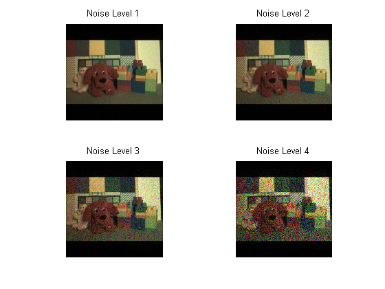 Fig. 2-2. Input images with different noise levels |
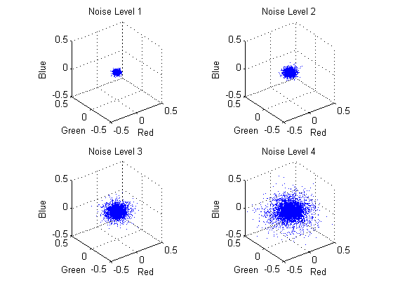 Fig. 2-3. 3D scatter error plots of the noise model |
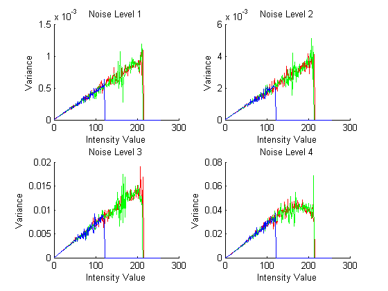 Fig. 2-4. v-i plots of the noise model |
|
We make several assumptions about our input noise. It follows Gaussian distribution for each intensity values. Also, it is white which means that noise does not have spatial correlation with neighboring pixels. Finally, there is no color channel correlation in input noise. These properties can be seen in Fig. 2-3. The RGB values of noise form sphere-shape point cloud in 3D RGB space since it does not have dependency in color values.
Input noise can be divided into additive noise and multiplicative noise as shown in Fig. 2-4. The additive noise and multiplicative noise can be represented by the affine model in variance-intensity plot. The y crossing tells additive noise term and the slope corresponds to the multiplicative noise term. As the noise level goes higher, we get larger slope because photon noise becomes the dominant factor in noise. The y crossing remains the same because readout noise is fixed by the sensor itself. In this model, multiplicative noise is the main factor in all cases and we are fine to assume that the additive term is very small compared to the other term. For the image with highest noise level, the plot bends in the end because the size of noise itself is limited by the maximum voltage allowed to a sensor pixel and saturated. |
| Demosaic Algorithm Analysis | Top |
| Demosaic Artifacts |
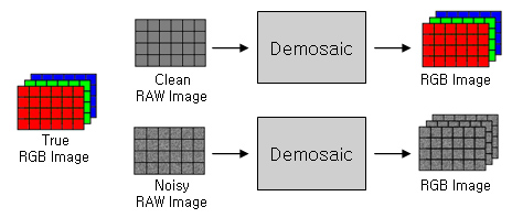 Fig. 2-5. Demosaic artifact test |
|
If we compare the noiseless ground truth RGB image with the demosaiced noiseless RAW format image, we can see the performance of demosaic algorithm itself without intervened by noise. Usually, demosaic algorithms cause several artifacts such as zipper effect and color artifact which are easily seen around edges and densely textured regions. The frequency orientation test pattern is good for observing errors with different frequency scale and orientation. Fig. 2-6 and 2-7 clearly show that bilinear demosaic algorithm introduces much color artifacts while other methods are better at suppressing color errors. Also, we can see that it is hard to deal with horizontal edges and vertical edges for all algorithms.
|
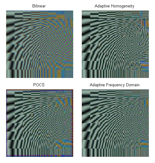 Fig. 2-6. The demosaiced results for frequency orientation test pattern |
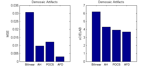 Fig. 2-7. MSE and sCIELAB comparisons for each demosaic algorithm |
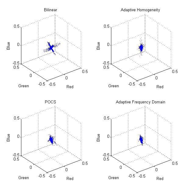 Fig. 2-8. 3D scatter plots for demosaic artifacts |
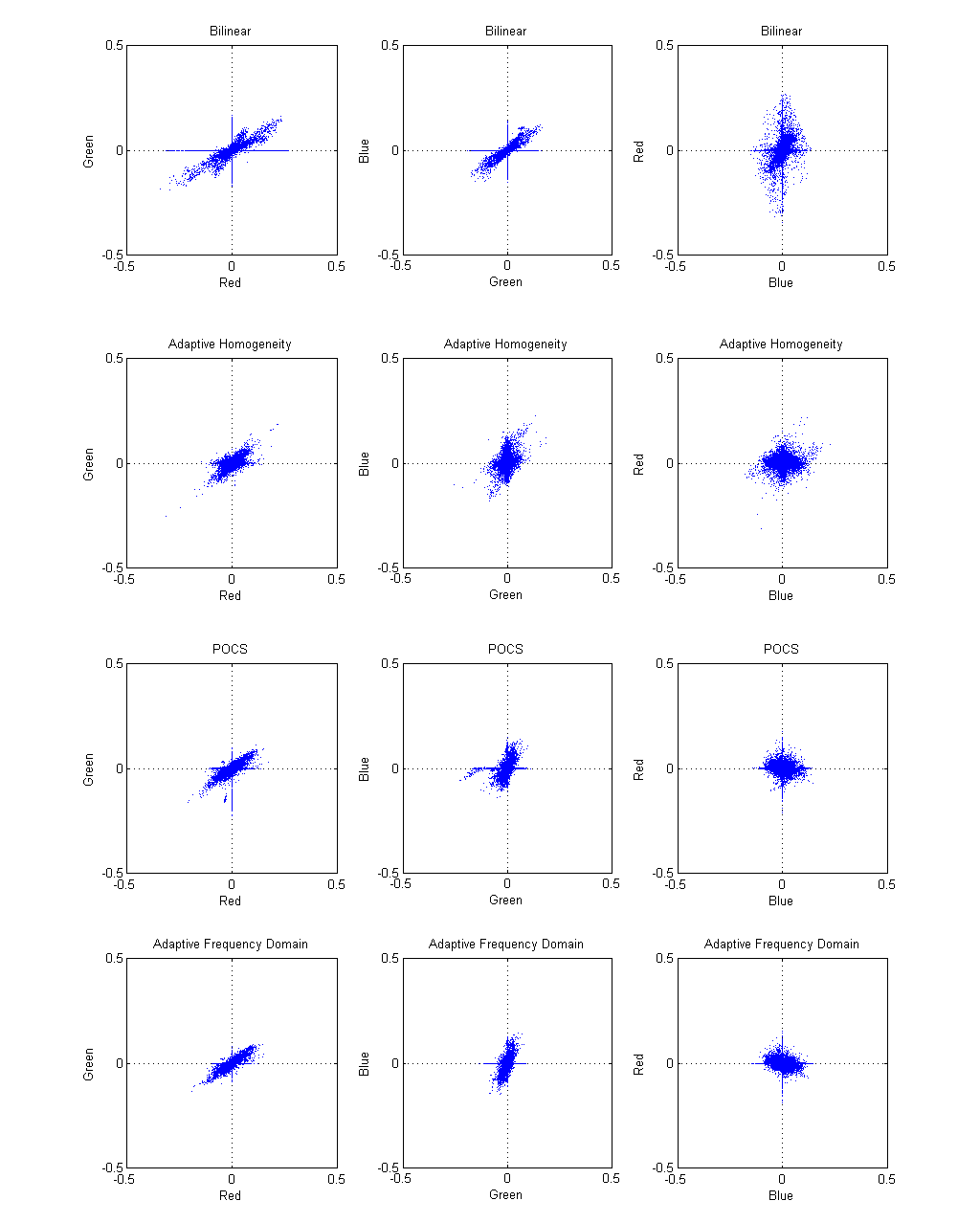 Fig. 2-9. The projects of 3D scatter plots onto 2D space |
|
Fig. 2.8 shows 3D scatter plots for demosaic artifacts and Fig. 2-9 is their projections to three 2D spaces to get better visualization. It is interesting to see that they have peculiar structure in error values. Except for adaptive homogeneity algorithm, we can see the big cross in the center of projected 2D space. This is caused by the fact that we have at least one correct value at each pixel because one value in some channel has been actually observed. At least a quarter of value in R and B channel is perfect and those points have error in 2D space. From the observation we can tell that adaptive homogeneity algorithm changes the value to make estimation even though the value is directly measured from the sensor. Another observation is that some point clouds are tilted to a certain direction. This is because we get much less error in green channel since we have twice many samples in green channel.
|
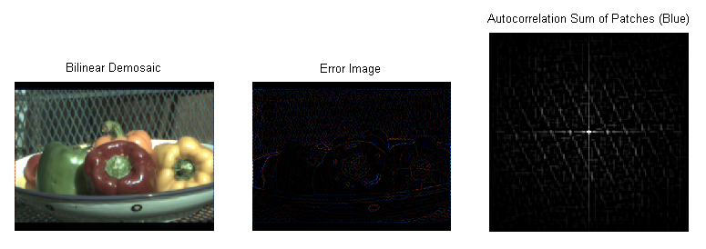 Fig. 2-10. Visualization of demosaic artifacts |
|
We can see where the demosaic artifacts occur in image from the error image plot in Fig. 2-10. Almost all errors are aligned with edges in the image. It implies that demosaic artifacts depends on input image characteristics. Also, if input image has some repeated patterns or textures, demosaic errors will have spatial correlation, too. The right plot in Fig. 2-10 is obtained by adding autocorrelation of many patches in the image and reveals the fence structure in the background.
|
| Noise Propagation in Demosaic Algorithm |
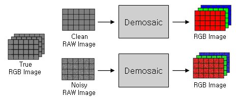 Fig. 2-11. Noise propagation test |
|
To see how noise propagates in demosaic process, we compare the demosaiced image of noiseless RAW image and demosaiced image of noisy RAW image since we already know the noise characteristics for input RAW image. From Fig. 2-12, noise distributions are stretched to one direction, deviated from the spherical shape clouds input. For bilinear method, the linear transform warped the sphere shape to the ellipsoidal form. Other algorithms result in much more stretched distribution to direction toward (1,1,1) and (-1,-1,-1). It means that noise become correlated within each color channel to from luminance noise. It can be understood that algorithms are doing a good job in suppressing color artifacts, which we can see from the above section.
|
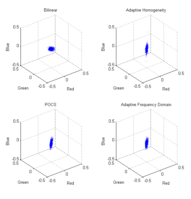 Fig. 2-12. 3D scatter plot after demosaic process |
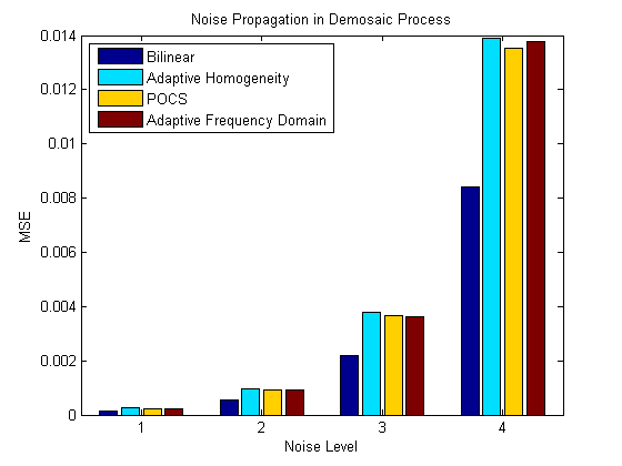 Fig. 2-13. Noise after demosaic process |
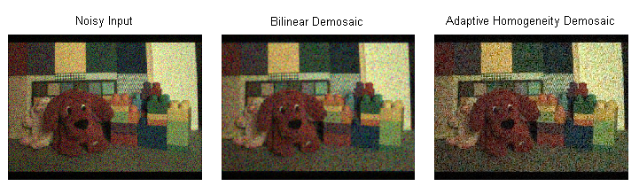 Fig. 2-14. Demosaiced images |
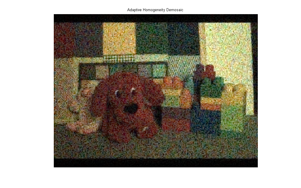 Fig. 2-15. The result image after adaptive homogeneity algorithm |
|
As you can see from Fig. 2-13, MSE of output image grows with input noise level. Other than bilinear methods are better at preserving high frequency details, but it may also boost noise component as well. Fig. 2-14 shows that demosaiced image can be very noisy when much noise is added to input image. Also, noise pattern becomes weird and seems to have spatial pattern. This makes denoising difficult.
|
| Input Noise and Demosaic |
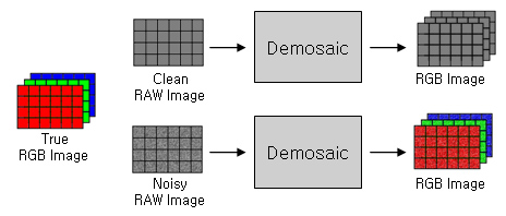 Fig. 2-16. Overall noise test |
|
We can compare the result of demosaic process of noisy input image to the ground truth RGB image in order to see the error to the image that we ultimately want. This error incorporates both demosaic artifacts and propagated input noise.
|
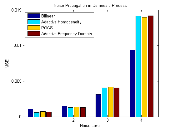 Fig. 2-17. The result image after adaptive homogeneity algorithm |
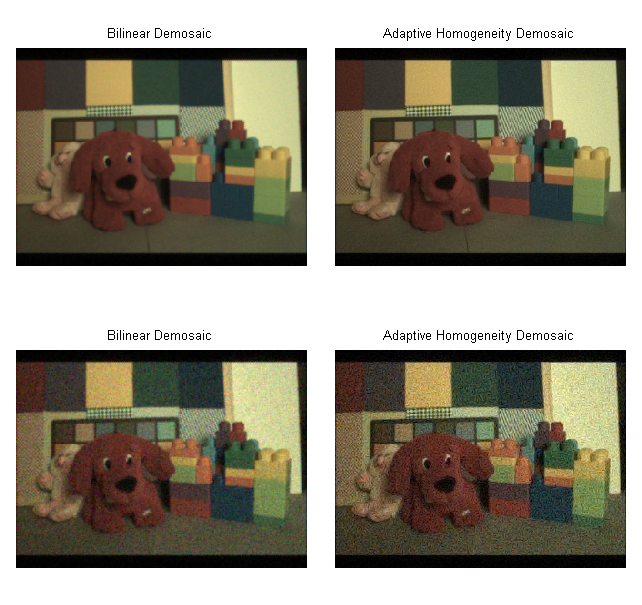 Fig. 2-18. The result image after adaptive homogeneity algorithm |
|
Fig. 2-17 and Fig. 2-18 clearly show this fact. When input noise level is low, complicate demosaic algorithms show better performance than simple bilinear interpolation. The images in Fig x show that the result is quite sharper and have lower MSE if we use good demosaic algorithm. However, as the noise input level goes up, complicated demosaic methods suffer from high noise and MSE grows faster than the bilinear case. The result images look noisier than the bilinear one which blurs noise out for some extent. As a results, we can conclude that demosaic artifact itself is dominant when input noise level is low, but noise caused by noisy input becomes more important as noise level goes high.
|
| Denoise Algorithm Analysis | Top |
|
Depending on the pipeline we may perform denoising on either a 3 channel RGB image, or the raw image itself. Most denoise algorithms work on 3 channel RGB images to leverage the low frequency characteristics of real world images. To denoise directly on RAW images one needs to either handle the Pattern created by the CFA array or perform denoising directly on the input signal without prior knowledge of the scene. If noise is spatially disjoint, as assumed in most cases, performing a single channel denoise on each channel can be justified.
|
| Denoise Algorithms for RGB Images |
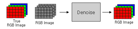 Fig. 2-19. Denoising for RGB images |
|
We tested the denoise algorithms on images with noise added into each channel. In Fig. 2-20 we see that at high nose levels bilateral filter seems to do good in both MSE and sCIELAB values. At lower levels BM3D tends to have lower sCIELAB values. It is worth noticing that a simple linear blur does well with MSE values and a moderately good job with sCIELAB values.
|
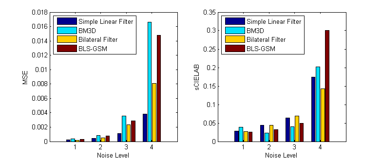 Fig. 2-20. Comparison of denoising algorithms |
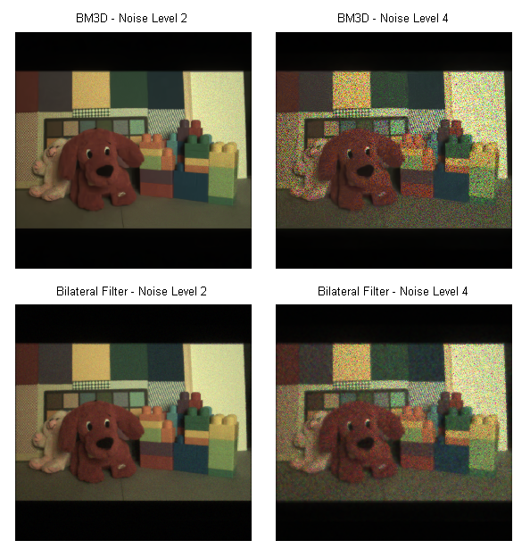 Fig. 2-21. The result images for high input noise level |
| Denoising on RAW Images |
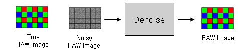 Fig. 2-23. Denoising for RAW images |
|
For the denoise-demosaic pipeline, the input for the denoise module will be a RAW image. Most denoise algorithms assume a 3 channel RGB image. To denoise the RAW image, we decompose the RAW image into each color channel. For the green channel we perform an additional interpolation. This process may itself effect the image quality or noise characteristics. It would be better to be able to denoise a RAW image directly. We have tried denoising a RAW image directly using BM3D. We believed the block matching algorithm of the BM3D should work directly on RAW images since it did not use spatial frequencies.
|
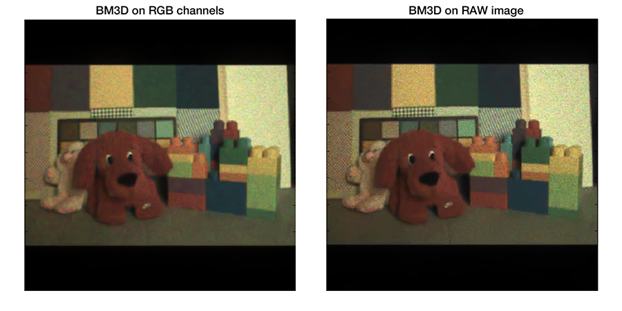 Fig. 2-23-1. BM3D applied to RGB and RAW images |
|
In Fig. 2-23-1 we see that BM3D seems to work on RAW images. But for some parts like the yellow patches it does not seem to denoise well. We are aware that the CFA pattern may affect the block matching, but the resulting seemed worth noting.
|
| Frequency Domain Analysis |
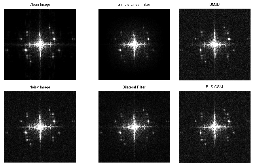 Fig. 2-22. Frequency domain representation of denoised images |
|
Denoising process is essentially a low-frequency filtering to remove high-frequency noise. The Fourier transform of noisy image shows that noise is uniformly spread all over the frequency domain, which is consistent with our assumption that noise is white. Simple linear filter is very effective at removing high frequency noise, but it blurs image much and looses fine detail in the original input. Other more complicated denoise algorithms are better in preserving details while reducing overall noise components.
|
| Demosaic-Denoise Pipeline | Top |
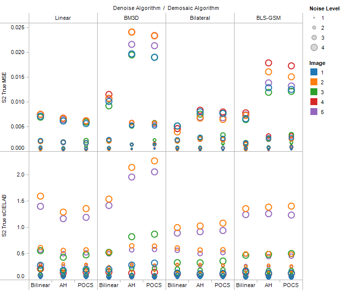 Fig. 2-24. Overall test results for demosaic-denoise pipeline |
|
This is the plot of MSE and sCIELAB values for different demosaic and denoise algorithms for the demosaic-denoise pipeline. An interesting observation can be made on how MSE values and sCIELAB values shoot up for the adaptive demosaic algorithms for BM3D in contrast to the simple bilinear interpolation method.
|
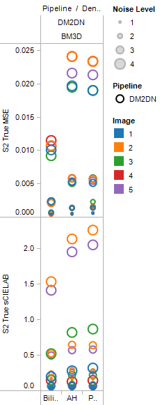 Fig. 2-25. BM3D in demosaic-denoise pipeline |
|
We investigated the reason for this behavior and found that adaptive homogeneity and POCS where structuring the noise in a way that BM3D could not handle.
|
| Demosaic Effects on Noise |
|
We saw in Demosaic Algorithm Analysis how the adaptive algorithms introduced correlation between color channels and changed the chrominance noise into luminance noise. This in turn seems to affected the BM3D algorithm.
|
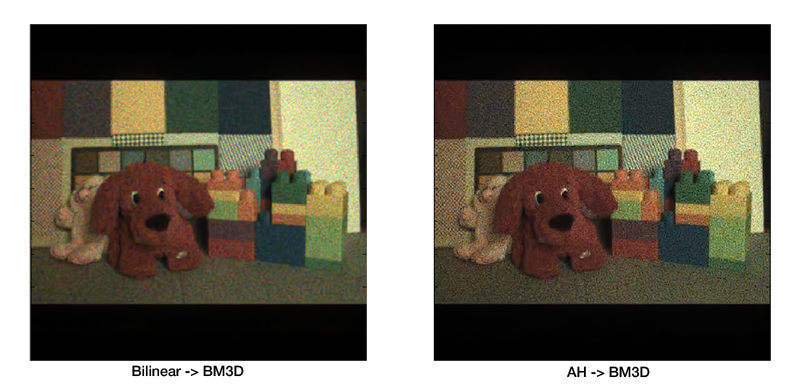 Fig. 2-25-1. The images after BM3D denoising with different demosaic methods |
|
These are the images of BM3D with different demosaic algorithms. The BM3D does not seem to do much with results from adaptive homogeneity.
|
| Luminance Noise and Color Noise |
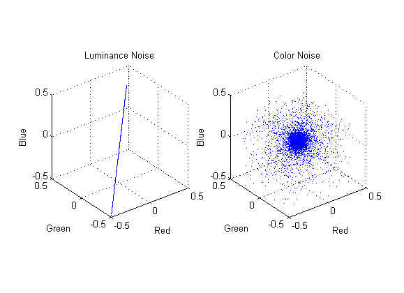 Fig. 2-26. 3D scatter plots of luminance noise and color noise |
|
Different noise characteristics to input images can affect the performance of denoising algorithms. Color channel correlation is one of the factors that can have influence in denoising. We applied luminance noise and color noise with the same variance, which are specific cases of color channel correlation. As you can see from Fig. 2-26, luminance noise has the same values in all RGB channels, while color noise has channel-independent noise that shown as a sphere-shape point clouds in 3D RGB space.
|
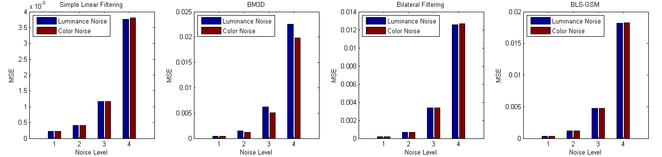 Fig. 2-27. The results of denoising for luminance noise and color noise |
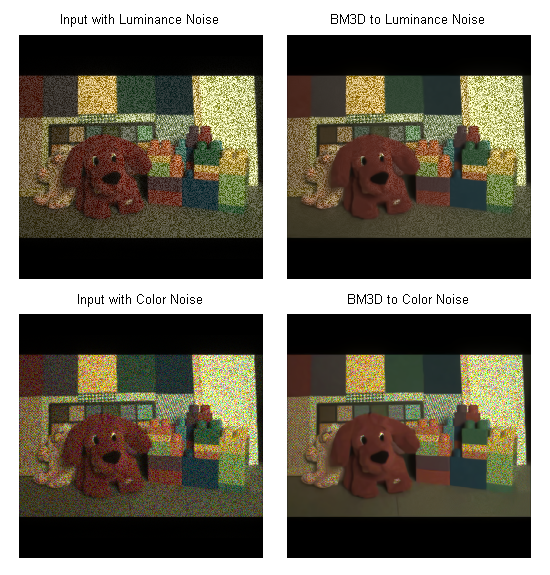 Fig. 2-28. The result images for luminance noise and color noise |
|
Our test result shows that performance of BM3D denoising algorithm depends on the character of input noise, while other methods show almost the same result. BM3D tends to have better result when channel-independent color noise is applied. In Fig. 2-28, the area of denoised region is much smaller when luminance noise is applied. This implies that BM3D was not able to find enough block matches to sum up in this case and denoising was not done effectively. Thus, we can conclude that denoising methods are actually affected by color channel correlation of input noise.
|
| Denoise-Demosaic Pipeline | Top |
|
According to our image pipeline, the scene goes through a CFA, gets transformed into an RGB scene and then sampled by an image sensor to a raw image. During the sampling process sensor noise is added due to the sensor characteristics. Undoing this process to estimate the original image would be to 1.denoise the raw image, then 2.demosaic a clean image.
Demosaic algorithms assume that the image is clean and the job for the algorithm is to interpolate the missing values correctly. The denoise algorithms job is to remove noise. Most denoise algorithms assume Gaussian noise based on sensor noise models. When we demosaic before denoise, the demosaic algorithm receives a noisy input with the assumption that there is no noise and in turn transforms the noise characteristics. The denoise algorithm then tries to remove noise with incorrect assumptions and, as the BM3D case in the previous section, does not denoise correctly. Denoising before demosaicking seems to be more natural. The denoising algorithm receives a noisy raw image and does its job. Next the demosaic algorithm receives a well denoised image and now performs demosaicking. |
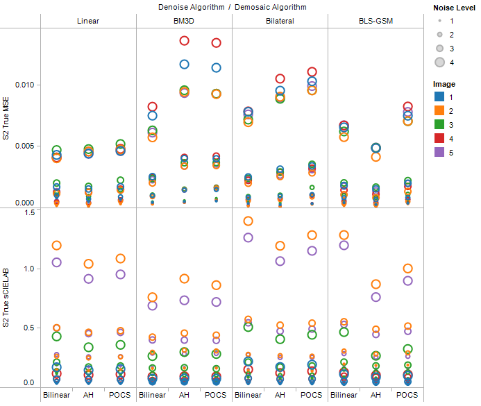 Fig. 2-29. Overall test results for denoise-demosaic pipeline |
|
This is the plots for different settings in the denoise-demosaic pipeline.
Though denoising before demosaicking may seem more intuitive, most denoising algorithms are designed to work on RGB images of grayscale images and not on RAW images. This becomes a problem because it requires manipulation on the RAW data to match the RGB format. It would be a challenge to find an algorithm that works directly on RAW images or develop such algorithms. |
| Joint Demosaic-Denoise | Top |
| Optimal Parameter Estimation |
|
Since the Joint Demosaic-Denoise algorithm uses the following noise model:
y(i,j)=x(i,j)+(k0+k1*x(i,j))n(i,j) y(i,j) is the noisy pixel value at (i,j); x(i,j) is the true pixel value at (i,j); n(i,j) is a random variable with distribution N(0,1); k0 is parameter for additive noise; k1 is parameter for multiplicative noise. To obtain an estimation for the two parameters k0 and k1, we need to investigate the image noise properties using the noise variance and intensity plot as below: |
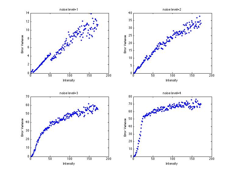 Fig. 2-30. V-I plots for parameter estimation |
|
As shown in the diagrams above, when the noise level is low, i.e: noise level=1 or 2, the noise variance and pixel intensity follows a strong positive linear correlation. Hence k0 and k1 can be easily obtained using the polyfit() function in Matlab.
However, for higher noise level, the linear relationship between error variance and pixel intensity start to break down. This is because the noise magnitude is assumed always less than the true pixel value. Therefore, when multiplicative noise facotr k1 is high, as the pixel value increases the the error variance starts to saturate. To obtain an accurate estimation for k0 and k1, the saturated part was truncated and the remaining data was pass into the polyfit() function. The results for different images are as shown below: |
| Image Name/Noise Level | Estimated k1 | Estimated k0 |
| Stuffed Animals | ||
| 1 | 0.0701 | 0.3072 |
| 2 | 0.2432 | 1.1705 |
| 3 | 0.7986 | 1.5410 |
| 4 | 2.3635 | -8.0144 |
| Morning Glory | ||
| 1 | 0.0708 | 0.1383 |
| 2 | 0.2540 | 0.6970 |
| 3 | 0.7687 | 1.9948 |
| 4 | 2.3145 | -7.3199 |
| Peppers | ||
| 1 | 0.0709 | 0.1424 |
| 2 | 0.2472 | 1.0608 |
| 3 | 0.7809 | 1.7671 |
| 4 | 2.3253 | -7.7206 |
| redrose | ||
| 1 | 0.0696 | 0.1473 |
| 2 | 0.2482 | 0.9952 |
| 3 | 0.7886 | 1.6681 |
| 4 | 2.4046 | -8.2016 |
| tomatos | ||
| 1 | 0.0717 | 0.0843 |
| 2 | 0.2448 | 1.0958 |
| 3 | 0.7885 | 1.4271 |
| 4 | 2.3143 | -7.4045 |
| optimal estimation | ||
| 1 | 0.07062 | 0.1639 |
| 2 | 0.2474 | 1.0038 |
| 3 | 0.7842 | 1.3625 |
| 4 | 2.3519 | -7.8141 |
|
Table 1. Estimated parameters for different input images |
|
Notice that within a reasonable range, the additive noise parameter k0 remains nearly constant for different noise level. The extra noise was contributed mainly by the multiplicative noise k1.This is consistent with the sensor model we adapted.
The optimal k0 and k1 value is obtained by the mean of the the k0 and k1 at the same noise level across different images.Note that k0 and k1 is noise parameters, they are independent to images. In other words, different images with the same noise level are expected to have the same k1 and k0 value. |
| Result Images |
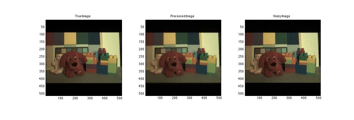 Fig. 2-31. The result images |
|
The result above shows the image with moderate noise added to the raw image. The calculated MSE of the image is 0.00095473 and the s-CieLab is 0.039861, which are relatively low. Though the image noise is shown effectively removed, the image also lose sharpness. In other words, the image loses high frequency details.
|
| The Algorithm Operation in the Frequency Domain |
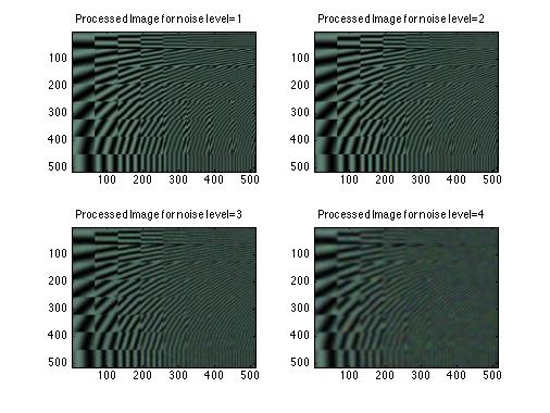 Fig. 2-32 . The result images for frequency orientation test pattern |
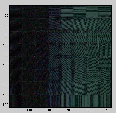 Fig. 2-33 . The error images for frequency orientation test pattern |
|
To explore the algorithm behaviour in the frequency domain, we apply the algorithm to the following test images under 4 different noise levels. As shown on the images above, when the noise levels increases from 1 to 4, the image sharpness deteriorate significantly. Intuitively, the algorithm is trading the image sharpness with grain noise. To see this property in more details, the difference image between the processed image at a moderate noise level and the true image. The result again confirms that the error is frequency dependent. Hence,to investigate how the algorith works in the frequency domain. We apply FFT on the error and compared to the equivalent RGB image noise.
|
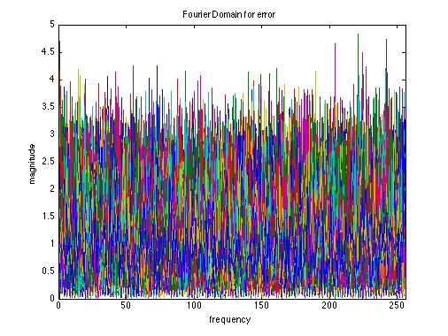 Fig. 2-34 . Fourier domain error before processing |
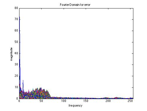 Fig. 2-35 . Fourier domain error after processing |
|
As shown in the results above, the joint Demosaic and Denoise algorithm is essentially a low pass filter to the noise. The total noise level is significantly reduced. However, if we compare the true image and the processed image in the frequency domain:
|
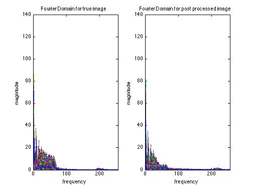 Fig. 2-36 . Fourier domain comparison |
|
It is notice that the high frequency components in the image is also filtered out, causing the image to blur. Hence as the image noise level increases, the pass band of the filter shrinks in order to effectively filter out the noise, it then at the same time filter out more high frequency components in the image, causing more severe blurring. Hence tuning the algorithm is to choose a compromise between "grain" noise and blur in image.
|
| The Algorithm Operation in Different Color Channels |
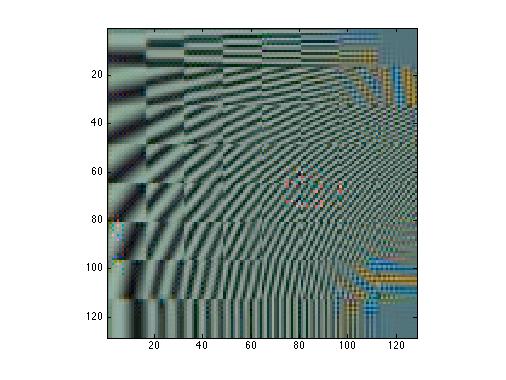 Fig. 2-37 . Processed clean raw image |
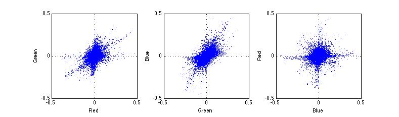 Fig. 2-38 . RGB error projection for processed clean raw image |
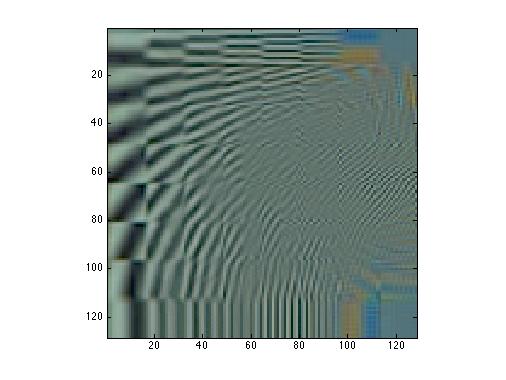 Fig. 2-39 . Processed noisy raw image |
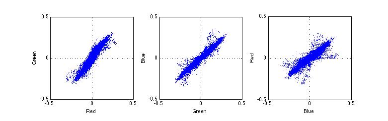 Fig. 2-40 . RGB error projection for processed clean raw image |
|
Fig 2-40 shows that the blue and red channel suffer from higher error, than the green channel. This is because the Bayer pattern used for the sensor has 2 time more green pixels than red or blue pixels. Hence the estimation for green pixels has a higher accuracy. Also notice the error scattering for R-B channel is close to a circle, meaning that the the error in the red and blue channels are uncorrelated. While the G-R and G-B error scattering suggests a linear relationship between the two errors. Also notice that when the noise level increases, the linear relationship becomes more evident.
|
| Summary |
|
To summarize, the joint Demosaic and Denosie algorithm can demosaic and remove the noise in the image effective. However, there is a trade off between noise cancellation and sharpness of the image in the algorithm. Also, the joint Demosaic and Denoise algorithm gives a more accurate estimation in the green channel than the red or blue channel, causing correlated noise between the G-B and G-R channel.
|
| Comparison Between Image Pipelines | Top |
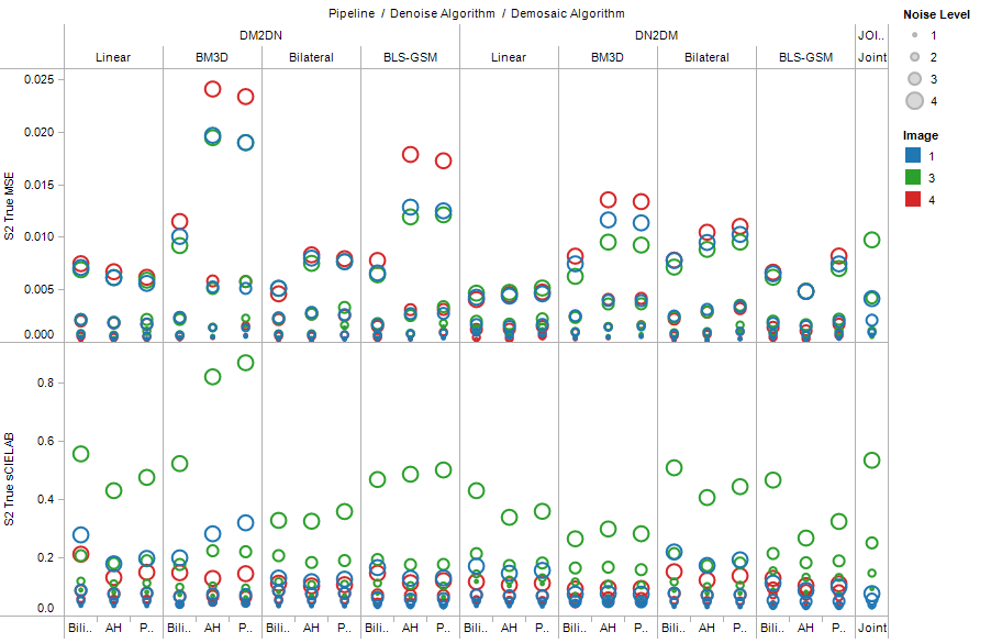 Fig. 2-41. Comparison of MSE and sCIELAB for each image pipeline |
|
This is the result of all pipelines. We cannot do a direct comparison between pipelines because each pipeline uses different parameters. However, we may do a simple qualitative comparison. The joint algorithm tends to have better results in both MSE and sCIELAB values. Denoising first seems to have lower MSE values but similar sCIELAB values to demosaicking first.
|
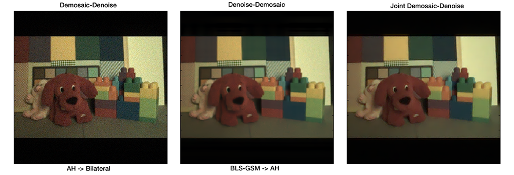 Fig. 2-42. Selected images from each image pipeline |
|
We've chose the images with the best tradeoff between MSE and sCIELAB values. Viewing the results we see that for the demosaic first case the luminance noise from the adaptive homogeneity is still visible. Denoising first seems to reduce this effect. The joint algorithms seem to do a good job of removing the noise. But, there are unwanted artifacts in the results. The joint algorithm seems to do a bad job in high-frequency regions mistaking detail for noise.
|