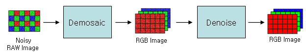
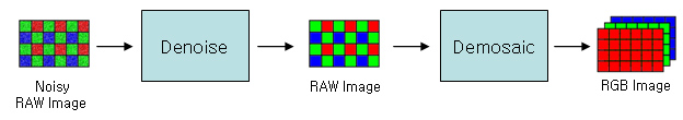
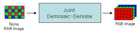
Fig. 1-1. Image pipelines: Demosaic-Denoise, Denoise-Demosaic, Joint Demosaic-Denoise
|
Evaluation of Noise Characteristics in Image Pipeline |
| Annabel Huo, Hyung Suk Kim, Sung Hee Park March 21, 2009 Psych 221 : Applied Vision and Image Systems |
| | Introduction | Methods | Results | Conclusions | References | Appendix | |
| Image Pipelines |
|
Fig. 1-1. Image pipelines: Demosaic-Denoise, Denoise-Demosaic, Joint Demosaic-Denoise |
|
Several kinds of image pipelines can be used to do demosaic and denoise operations. All pipelines get RAW format images as input and returns RGB color images. The first pipeline in Fig. 1-1 is the most commonly used image pipeline to do this. However, we can consider another image pipeline with different order of operations as you can see in Fig. 1-1. Also, joint demosaic-denoise pipeline can be used to do the same operation efficiently.
To evaluate and test each image pipeline, we have built our own image pipeline so that the quality of output images and noise properties can be characterized in each stage. Our image pipeline consists of image acquisition module, demosaic module, denoise module, joint demosaic-denoise module, image-noise evaluation module and data analysis module as shown in Fig. 1-2. |
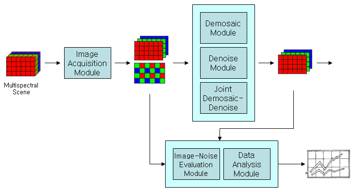 Fig. 1-2. Overview of image pipelines design |
| Image Acquisition Module |
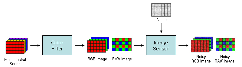 Fig. 1-3. Image acquisition module |
|
Image acquisition module uses ISET to acquire various images from multi-spectral scenes. By changing various settings, we get perfect RGB images with no noise, which are used as ground truth reference image, along with multiple test images with different noise levels.
A perfect RGB image is generated by compositing three images captured with red, green, and blue color filters, having all RGB values in each pixel. This image can be sampled to make a RAW format image which corresponds to CFA pattern of our choice, such as well-known RGB Bayer pattern. Noise can be added to simulate artifacts we can see in real photographs. Photon noise, readout noise, dark signal non-uniformity, pixel response non-uniformity and so on are controlled separately, which can be modeled as additive noise and multiplicative noise. To get different levels of noise, we change conversion gain in the sensor and exposure time since they give the same effect as changing ISO speed in photography. |
| Demosaic Module |
|
| Denoise Module |
Denoise algorithm can be applied to both RGB image and RAW format image. For RGB images denoising is done for each channel separately and combined. For RAW format images, input image is decomposed first. Red pixels are collected to form a red channel image without any blank to form an image of a quarter sizes. Same operation is done for blue pixels. Green pixels are interpolated to have a green channel image that is the same size as the original input so that spatial relationships between pixels are not disturbed. After denoising each channel, they are sampled and combined again to form a RAW format image. |
| Joint Demosaic-Denoise Module |
| Joint Demosaic-Denoise use TLS (Total Least Squares) |
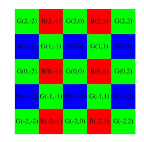 Fig. 1-4. A filter window for joint demosaic-denoise algorithm |
|
The Joint Demosaic-Denoise module implemented in this project was built based on the TLS denoise algorithm. A denoise filter was designed to optimally estimate a pixel value from a noisy single-color image(the raw image). By adding some constrains to the filter, the filter is also optimal for demosaic. Then the image is processed in a 5X5 window as shown in Fig. 1-4. As shown in Fig. 1-4, we are trying to estimating the ideal central pixel value G(0,0) using the noisy pixel information in the window, using the following method:
G(0,0)=sum(a(i,j)Y(i,j)) a(i,j) is the filter coefficients; Y(i,j) is the noisy pixel values in the window. By assuming that the difference images between the RGB channels are band limited, hence we can assume that the low frequency components at each color planes are dissimilar, but the high frequency components at each planes are similar. Thus we need to choose a(i,j), such that it is a high pass filter in the R, B plane, and it also estimates the ideal G(0,0) value from G(2i,2j). In theory, any denoise algorithms which also satisfy the above constraint can build a joint denoise and demosaic filter. In this project the TLS denoise algorithm is applied. The algorithm assumed that the RAW image is quantized to 8-bit unsigned integers (0~255). |
| Estimating the Optimal Parameters |
|
The joint Demosaic-Denoise TLS algorithm was suggested to optimize the two stages simultaneously from the two input parameter k0 and k1, which relates the noise model for the sensor:
Y(i,j)=x(i,j)+(k0+k1x(i,j))n(i,j) n(i,j)~norm(0,1) :k0:parameter for additive image :k1:parameter for multiplicative image The parameters k0 and k1 are usually provided by the manufacturers. In this project they are estimated from the error variance and intensity plot. |
| Image-Noise Evaluation Module |
|
| Data Analysis Module |
|
With 7 images, 4 noise levels, 4 demosaic algorithms, 4 denoise algorithms, and 2 different orders we had almost 900 different settings to visualize. It would be too time consuming to generate and view 900 images, along with another handful of error plots, so we looked at the MSE and sCIELAB values to obtain an overview of the data. We used Tableau, a data visualization software for creating plots and explored the data set to find points of interest. Then based on the data plot, we obtained the image with the settings of interest.
|