Optimizing
Scanning Filters For Color Balanced Multispectral Image Recovery
Dinesh
Baniya
Applied
Vision and Imaging Systems
1)
Motivation
In order to obtain color balanced
spectral measurements from a multispectral system, it is necessary to choose optimum
sensors or filters for the task for which a multispectral system has been
designed. Computer simulations of the spectral sensitivity of sensors and their
response to spectral information with varying levels of noise will provide
insight to the quality of the spectral power density (SPD) curves that can be
recovered. If these computational models simulate the real world accurately
enough, the information provided by them will be extremely useful in the design
and fabrication of sensors for a multispectral imaging system.
2)
Introduction
In recent years the development
of multispectral color-image acquisition instruments has received much
attention in the field of color science. An optimum multispectral system must
estimate the spectral radiance at each pixel of the image based on the response
of the system’s channels. This is a classic inverse problem that requires a
mathematical estimation algorithm. In this project I have used a linear model
based on Wiener’s method. Not all mathematically realizable sensors are
physically realizable, so the simulated system must model the behavior of realistic
optimum sensors. To incorporate a manageable dynamic range and smoothness for physically
realizable filters, I have used Gaussian functions. Any search for an optimum set of Gaussian
sensors (those whose spectral sensitivities are Gaussian functions of
wavelength) intended to recover a multispectral image depends on several
factors: the spectral response of its sensors, the type and number of sensors,
and the noise that always affects any electronic device. To include all these
factors in an exhaustive search is a highly demanding computational task. An alternative
approach that greatly reduces computing time is to minimize a single cost
function, and for this project I have used a calorimetric cost function. The
multispectral dataset obtained from Intuitive Surgical was used to test the
accuracy of the simulated sensors.
3)
Design
Approach
As far as the spectral estimation
method is concerned, it must be clear from the beginning that extracting
spectral information in the visible range from the responses of a few sensors
is an under-dimensioned mathematical problem because the projection of the spectra
in the sensor-response space leads to a substantial loss of information. Various
mathematical algorithms exist that allow the estimation of spectral information
from sensor responses. Some of the methods tried in various literatures are the
Maloney–Wandell method, the Imai–Berns method, the Shi–Healey method, and the
Wiener method. These methods are commonly based on a priori knowledge of
the kind of spectra that is to be recovered. In this project I have used the Wiener
method to estimate spectral information.
In the Wiener approach, the
original multispectral image is denoted by (x). Then an equation of the form y
= Ax + n can be formed where (A) is a matrix formed by the product of the
illuminant SPD and the sensor SPD and (n) represents the photon/shot noise. The
estimated spectra is denoted by (x’) and is obtained via the equation x’ = W *
y, where W is the Wiener parameter and is represented by W = (Rxx *
AT) * (A * Rxx * AT+ VN)-1.
In this expression Rxx
denotes the autocorrelation of (x) and VN denotes the variance of
the noise.
Once
the estimation algorithm has been chosen the next step is to select
mathematical functions that can represent physically realizable filters. The
filters need to be smooth and nonnegative. Some of the functions that have been
tried are Gaussian and raised Cosines. For this project I have picked Gaussian
functions. Furthermore, the sensors need to have a certain SPD. The SPD of the
sensors is dictated by the SPD of silicon. The SPD of silicon falls off sharply
towards the blue region of the spectrum, but has a long tail that extends out
into the IR region.
|
Figure 1: The
SPD of Silicon |
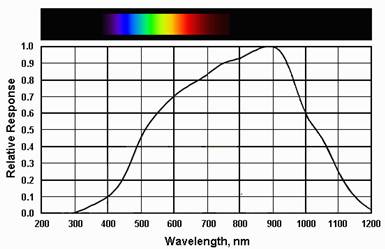
In order to conform to the SPD of
silicon, I have designed the Gaussian functions to have a broad standard
deviation when their means fall towards the red region of the spectrum and a
narrower standard deviation when their means fall in the blue end of the
spectrum.
A Gaussian function is
characterized by its mean and standard deviation. Since the sensors need to
operate in the visible region of the spectrum, the means can vary from 400 nm
to 700 nm. The standard deviation is arbitrary and I have chosen their range to
be 1 nm to 100 nm. The amplitudes of the Gaussian functions are kept constant
at unity.
An optimum set of Gaussian
sensors given by the above design space via an exhaustive search is a
computationally intensive task. In order to compute the results within a
reasonable time frame, I have chosen a cost function that needs to be minimized.
Since this project focuses on color balancing, I have based the cost function
on calorimetric metrics such as those proposed by CIELAB. These metrics
approximate color differences observed by the human eye.
Optimization of the filters was
done using the “fmincon” function of MATLAB. This function attempts to find
local minima of multivariable functions given a set of constraints and an
initial condition. This function is not guaranteed to find the global minimum,
however it provides local minima values based upon the starting condition. For
this project I wrote the code so that the function begins with 50 different
initial conditions chosen at random. The initial conditions are the numbers of
filters to be used and the values for the mean and standard deviation for each
filter. The constraints are the ranges for the mean and standard deviation. So
starting from 50 different initial conditions the algorithm provided 50
different estimates for the cost function. These values were within 5% of each
other. I picked the filter combination that provided the lowest value for the
cost function.
Throughout the simulation process I have kept the
illuminant SPD constant and the illuminant is Tungsten. The spectra used for
this project was obtained from Intuitive Surgical.
|
Figure 2: The
SPD of Tungsten illuminant |
Figure 3: Original Spectra |
4)
Results
I have created three sensors each having different
number of filters. The first one has only 2 Gaussian filters, the second one
has 3 Gaussian filters and the third one has 4 Gaussian filters. I have
compared them against the performance of a NikonD100 sensor. The simulations
were performed under both high (40 dB) signal-to-noise-ratio (SNR) and low (20
dB) SNR conditions.
Case
1a: NikonD100
sensor with SNR = 40 dB
|
Figure
4: Blue curves shows transmission of sensor and red curve shows RMSE between
original and estimated spectra |
Figure
5: Distance metric in CIELAB for each surface |
|
Figure
6: Surface with the maximum distance metric in CIELAB |
Figure
7: Surface with the minimum distance metric in CIELAB |
From figure 4 it can be seen that the NikonD00
sensor uses 3 filters. Also the peaks of the filter transmission correspond to
dips in the RMSE plot. This shows that the minimum error occurs when the filter
transmission is the highest. The distance metric in CIELAB for each surface is
shown in figure 5. Figure 6 shows the surface having the largest distance
metric (5.3974) in CIELAB, the solid line is the original spectrum and the
dashed line is the estimated spectrum. Similarly figure 7 shows the surface having
the smallest distance metric (0.1037) in CIELAB, the solid line sis the
original spectrum and the dashed line is the estimated spectrum.
Case
1b: NikonD100
sensor with SNR = 20 dB
|
Figure
8: Blue curves shows transmission of sensor and red curve shows RMSE between
original and estimated spectra |
Figure
9: Distance metric in CIELAB for each surface |
|
Figure
10: Surface with the maximum distance metric in CIELAB |
Figure
11: Surface with the minimum distance metric in CIELAB |
When the SNR is reduced from 40 dB to 20 dB, it can
be seen from figure 8 that the filter transmission peaks are no longer aligned
with the dips in the RMSE plot. This could be because the Wiener method is
linear and the addition of too much noise has caused the algorithm to make
misguided estimate. The distance metric in CIELAB for each surface is shown in
figure 9. Figure 10 shows the surface having the largest distance metric
(15.0848) in CIELAB, the solid line is the original spectrum and the dashed
line is the estimated spectrum. Similarly figure 11 shows the surface having
the smallest distance metric (1.1151) in CIELAB, the solid line sis the
original spectrum and the dashed line is the estimated spectrum.
Case
2a: 2 Gaussian
filters with SNR = 40 dB
|
Figure
12: Mean distance metric in CIELAB versus the number of iterations of
minimizing function |
Figure
13: Blue curves shows transmission of sensor and red curve shows RMSE between
original and estimated spectra |
|
Figure
14: Surface with the maximum distance metric in CIELAB |
Figure
15: Surface with the minimum distance metric in CIELAB |

Figure 12 shows the number of iterations the
minimization function has to make in order to reach a stable value for the mean
distance metric (3.3) in CIELAB across all 70 surfaces of the spectra. Figure
13 shows two Gaussian filters that make up the sensor, and the peaks of the
filter transmission correspond to dips in the RMSE plot. This shows that the
minimum error occurs when the filter transmission is the highest. Figure 14
shows the surface having the largest distance metric (16.8706) in CIELAB, the
solid line is the original spectrum and the dashed line is the estimated
spectrum. Similarly figure 15 shows the surface having the smallest distance
metric (0.2654) in CIELAB, the solid line sis the original spectrum and the
dashed line is the estimated spectrum.
Case
2b: 2 Gaussian
filters with SNR = 20 dB
|
Figure
16: Mean distance metric in CIELAB versus the number of iterations of
minimizing function |
Figure
17: Blue curves shows transmission of sensor and red curve shows RMSE between
original and estimated spectra |
|
Figure
18: Surface with the maximum distance metric in CIELAB |
Figure
19: Surface with the minimum distance metric in CIELAB |
Figure 16 shows the number of iterations the
minimization function has to make in order to reach a stable value for the mean
distance metric (4.1) in CIELAB across all 70 surfaces of the spectra. Figure 17
shows two Gaussian filters that make up the sensor. When the SNR is reduced
from 40 dB to 20 dB, it can be seen from figure 17 that the filter transmission
peaks are no longer aligned with the dips in the RMSE plot. This could be
because the Wiener method is linear and the addition of too much noise has
caused the algorithm to make misguided estimate. Figure 18 shows the surface having the largest
distance metric (17.6832) in CIELAB, the solid line is the original spectrum
and the dashed line is the estimated spectrum. Similarly figure 19 shows the
surface having the smallest distance metric (0.5136) in CIELAB, the solid line
sis the original spectrum and the dashed line is the estimated spectrum.
Case
3a: 3 Gaussian
filters with SNR = 40 dB
|
Figure
20: Mean distance metric in CIELAB versus the number of iterations of
minimizing function |
Figure
21: Blue curves shows transmission of sensor and red curve shows RMSE between
original and estimated spectra |
|
Figure
22: Surface with the maximum distance metric in CIELAB |
Figure
23: Surface with the minimum distance metric in CIELAB |
Figure 20 shows the number of iterations the
minimization function has to make in order to reach a stable value for the mean
distance metric (0.5) in CIELAB across all 70 surfaces of the spectra. Figure 21
shows three Gaussian filters that make up the sensor, and the peaks of the
filter transmission correspond to dips in the RMSE plot. This shows that the
minimum error occurs when the filter transmission is the highest. Figure 22
shows the surface having the largest distance metric (1.2954) in CIELAB, the
solid line is the original spectrum and the dashed line is the estimated
spectrum. Similarly figure 23 shows the surface having the smallest distance
metric (0.1429) in CIELAB, the solid line sis the original spectrum and the
dashed line is the estimated spectrum.
Case
3b: 3 Gaussian
filters with SNR = 20 dB
|
Figure
24: Mean distance metric in CIELAB versus the number of iterations of
minimizing function |
Figure
25: Blue curves shows transmission of sensor and red curve shows RMSE between
original and estimated spectra |
|
Figure
26: Surface with the maximum distance metric in CIELAB |
Figure
27: Surface with the minimum distance metric in CIELAB |
Figure 24 shows the number of iterations the
minimization function has to make in order to reach a stable value for the mean
distance metric (2.7) in CIELAB across all 70 surfaces of the spectra. Figure 25
shows three Gaussian filters that make up the sensor. When the SNR is reduced
from 40 dB to 20 dB, it can be seen from figure 25 that the filter transmission
peaks are no longer aligned with the dips in the RMSE plot. This could be
because the Wiener method is linear and the addition of too much noise has
caused the algorithm to make misguided estimate. Figure 26 shows the surface having the
largest distance metric (7.8050) in CIELAB, the solid line is the original
spectrum and the dashed line is the estimated spectrum. Similarly figure 27
shows the surface having the smallest distance metric (0.4282) in CIELAB, the
solid line sis the original spectrum and the dashed line is the estimated
spectrum.
Case
4a: 4 Gaussian
filters with SNR = 40 dB
|
Figure
28: Mean distance metric in CIELAB versus the number of iterations of
minimizing function |
Figure
29: Blue curves shows transmission of sensor and red curve shows RMSE between
original and estimated spectra |
|
Figure
30: Surface with the maximum distance metric in CIELAB |
Figure
31: Surface with the minimum distance metric in CIELAB |
Figure 28 shows the number of iterations the
minimization function has to make in order to reach a stable value for the mean
distance metric (0.39) in CIELAB across all 70 surfaces of the spectra. Figure 29
shows four Gaussian filters that make up the sensor, and the peaks of the
filter transmission correspond to dips in the RMSE plot. This shows that the
minimum error occurs when the filter transmission is the highest. Figure 30
shows the surface having the largest distance metric (1.1033) in CIELAB, the
solid line is the original spectrum and the dashed line is the estimated
spectrum. Similarly figure 31 shows the surface having the smallest distance
metric (0.05602) in CIELAB, the solid line sis the original spectrum and the
dashed line is the estimated spectrum.
Case
4b: 4 Gaussian
filters with SNR = 20 dB
|
Figure
32: Mean distance metric in CIELAB versus the number of iterations of minimizing
function |
Figure
33: Blue curves shows transmission of sensor and red curve shows RMSE between
original and estimated spectra |
|
Figure
34: Surface with the maximum distance metric in CIELAB |
Figure
35: Surface with the minimum distance metric in CIELAB |
Figure 32 shows the number of iterations the
minimization function has to make in order to reach a stable value for the mean
distance metric (2.3) in CIELAB across all 70 surfaces of the spectra. Figure 33
shows four Gaussian filters that make up the sensor. When the SNR is reduced
from 40 dB to 20 dB, it can be seen from figure 33 that the filter transmission
peaks are no longer aligned with the dips in the RMSE plot. This could be
because the Wiener method is linear and the addition of too much noise has
caused the algorithm to make misguided estimate. Figure 34 shows the surface having the
largest distance metric (8.3124) in CIELAB, the solid line is the original
spectrum and the dashed line is the estimated spectrum. Similarly figure 35
shows the surface having the smallest distance metric (0.5223 in CIELAB, the
solid line sis the original spectrum and the dashed line is the estimated
spectrum.
I have summarized the findings from above in the
tables below.
When the SNR is high adding more filters decreases
the mean metric distance in CIELAB.
However when the SNR is low the Wiener approximation
fails and the results are unpredictable. The trend that adding more filters
decreases the mean metric distance in CIELAB still continues. Comparing the
data from the two tables it can be seen that by decreasing the SNR, the mean
metric distance increases for the same number of filters.
5)
Conclusion
In this project I have
attempted to optimize scanning filters for accurate color balanced
multispectral image recovery. The Wiener method was used to estimate the
spectra and Gaussian functions were used to create sensors that optimized the
distance metric in CIELAB which formed the cost function. The optimization was performed
using the “fmincon” function of MATLAB and results from 2, 3, 4 Gaussian
filters were compared with the performance of a NikonD100 sensor. It was found
that when the SNR is high, the sensors performed really well and by increasing
the sensors the distance metric in CIELAB decreased. However, when the SNR was reduced the Wiener
approximation failed and the sensors did not perform as expected.
6)
Acknowledgements
I would like to thank the following people for their
help in this project.
Professor Brian Wandell
-
Teaching
the basics of color and vision systems
Dr. Joyce Farrell
-
Project Formulation/Counseling
-
Multispectral data collection
arrangement with Intuitive Surgical
Steven Lansel
-
Project guidance
-
Multispectral data collection at
Intuitive Surgical
-
Weekly meetings
-
MATLAB help
Jeff DiCarlo
-
Contact person at Intuitive Surgical
-
Multispectral data collection at
Intuitive Surgical
7)
References
[1] Miguel Lopez-Alvarez,
et.al “Selecting algorithms, sensors, and linear bases for optimum spectral
recovery of skylight”, JOSAA, Vol. 24, Issue 4, 2007
[2] Miguel Lopez-Alvarez,
et.al, “Designing a practical system for spectral imaging of skylight”, Applied
Optics, Vol. 44, No. 27, 2005
[3] Manu Parmar and
Stanley Reeves, “Optimization of Color Filter Sensitivity Functions for Color
Filter Array Based Image Acquisition”, 2006
[4] Poorvi L. Vora and H.
Joel Trussell, “Mathematical Methods for the Design of Color Scanning Filters”,
IEEE Transactions on Image Processing, Vol. 6, No. 2, 1997
8)
Links