Color Loader
Psych 221 Final Project
Daniel Chang, Winter 2009
Introduction
Have your picture.s colors ever turned out weird, even though the scene looked perfectly normal when you took it? The issue at hand is one of color balancing. Humans have color constancy . that is, the human color perception system maintains a relative relation between colors that helps them look constant under any light. To a person, an apple looks red in the broad daylight, as it will under a blue light. However, if you took a picture of a red apple under blue light and displayed the picture on a monitor, the apple will likely look purple. Unlike humans, cameras do not maintain color constancy, and hence pictures may look off-color.
The challenge of color balancing is to take a picture . with unknown surfaces and unknown illuminants . and .fix. it back to what a human observer might observe under D65 light (daylight). Because the camera sensor that captures the picture, the surfaces in the picture, and the light that shines on the surfaces do not match a .normal. observed scene to humans, color balancing is often an essential step in displaying digital photographs.
Motivation
While this project does not directly implement a color balancing algorithm, the motivation is to provide an interactive database that illustrates the importance of color balancing, and which can aid in testing color balancing algorithms.
To test a color balancing algorithm, a vision scientist will need spectral data of different surfaces, lights, and cameras. With this data, they can test to see if their color balancing algorithm can adequately restore a scene to its ideal representation. Thus, a web database carrying all this spectral information would have many practical purposes. However, even though web databases of surface reflectances, illuminant spectral power distributions, and camera RGB responses do exist, most of them are static databases containing text files, which have limited usability [1][2][3].
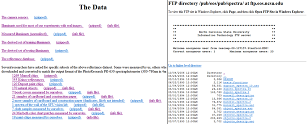
These websites contain useful spectral data, but the user cannot interact with the data outside of browsing through each link and getting numerical text files. The users cannot represent each scene visually nor see how lights, cameras, and surfaces interact with each other. Text data is a non-intuitive way of representing information . an interactive, visual database would greatly improve upon what currently exists.
The objective of this project was to provide a web utility and database that accomplish two key things:
- Data transparency . the data is stored in the back-end, but an end user can easily access the raw spectral data if she desires. This is helpful for testing color balancing algorithms. Additionally, the user can create and upload his own datasets (provided they are properly formatted) and load them into the web utility.
- Interactivity . Let the user exercise greater control and understanding over the data: filter and choose the data you want with easy-to-use user interface widgets. Display the RGB representation of the surfaces, illuminated by a user-specified light, and taken with a user-specified camera. Compare that on screen to an .ideal. representation that is properly color balanced. Grab the resultant RGB data of the scene.
Methods
Data Preprocessing
Before the database and utility were created, I needed raw spectral data . reflectances of surfaces, SPDs of lights, and RGB sensor responses of cameras . in order to build the data to be used and displayed. The data was gathered from text files in an online database [1][4] as well as ImagEval.s ISET utility [5]. Because the description of the data.s items and the actual numerical values were separate, manual creation of datasets was necessary to create usable data. This data was then formatted and parsed to be integrated into the web utility.
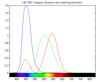
Above figure: to give an idea of what the spectral data are, imagine sampling these SPDs at 4 nm intervals, starting at 380 nm and ending at 784 nm. As another example, they could be sampled at 1 nm intervals, starting at 400 nm and ending at 760 nm. These data points comprise the spectral data for sensors, lights, or surfaces. The datasets used in my utility are basically sampled versions of reflectance functions, SPDs, and sensor responses.
Data Parsing
I constructed three datasets . one for the cameras, one for lights, and the last one for surfaces. The format of the data was chosen to facilitate the utility.s reading and understanding of the data, as well as the ease with which future users can create their own data. The format is described below, with the left column illustrating the conceptual format, and the right column being an example usage:
| # comments | # this is a comment preceded by a pound sign |
| Dataset_type | SURFACES,,, |
| #items, nm_step, nm_start, nm_end | 200, 4, 380, 784 |
| Item_name | BananaPeel,,, |
| Item_description | A yellow peel of banana,,, |
| Spectral_data | 0.01,,, |
| 0.23,,, | |
| ... | |
| 0.00,,, | |
| Next_item_name | RedApple,,, |
| Next_item_description | A Red Delicious apple,,, |
| Spectral_data | 0.37,,, |
| ... |
The first few lines of the data can be comments, provided each and every line starts with a # sign. Notice there are many extra commas in this data file . the data is comma delimited, and while the extra commas aren.t necessary, building the dataset in Excel and saving as CSV (comma delimited) will result in these commas. All valid data files are comma delimited (this is important for lines with multiple columns of data such as .200,4,380,784.).
Once the # signs end, the parser begins to recognize the text lines as important. The first meaningful line of each data set denotes the type of data in this file. Acceptable values are .SURFACES., .CAMERAS., and .LIGHTS..
The second line denotes important information about the file as a whole (these must be whole numbers). The first number is the number of items in this dataset, the second number is the interval of wavelength in nm for the data, the third number is the starting wavelength, and the fourth is the ending wavelength. In our example, .200,4,380,784. means there are 200 surfaces, and each surface has reflectance data starting from 380 nm, incrementing at 4 nm steps, and ending at 784 nm. You can enter any starting and ending wavelengths from 360 to 800 nm, and at a minimal interval of 1 nm.
After these two lines, the items themselves are stored. Each item has 2 lines for name and description, and sufficient lines as necessary for spectral data. In our example, each item has 1 line for its name (.BananaPeel.), 1 line for its description (.A yellow peel of banana.), and 101 lines for spectral data (this is from (784 nm . 380 nm) / 4 nm). After the spectral data of one item ends, the next immediate line begins another item.
The end of file is not signified. Based on the number of items indicated in line 2, the parser will recognize when to stop. If the user wishes to create his own datasets, this formatting must strictly be adhered to, or the parser will not understand the data. All lights, cameras, and surfaces datasets must also use the same starting, ending, and interval wavelengths, or matrix dimensions will not match.
In addition to loading spectral data from the web, the utility itself will construct the XYZ matching function in a matrix, with minimum wavelength 360 nm and maximum wavelength 800 nm, at 1 nm intervals. Based on the starting, ending, and interval wavelengths of the user.s datasets, the parser will construct the XYZ matrix to match these dimensions.
After the data are loaded, they are stored in matrices. When the user selects specific lights, cameras, and surfaces, the matrices are used to create the RGB representation of the scene.
Interaction - UI Widgets
To implement interactivity, I chose to develop my application in Java, using the JApplet and Javax.swing library. Rather than hard-coding the layout, I used the JApplet Form which allows GUI placing of Javax widgets. Currently JDK 6 is not compatible with Mac-OSX, so the application will not run on Macintosh computers.
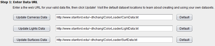
A major objective of this project is data transparency and enabling user-generated data. This is made possible with a UI widget that allows users to enter web URLs for their own data, while providing accessible default data they could examine as templates. To implement this, I let the users enter URLs in a text box and added a button that reads the data file at the URL. There is also a default button feature that reverts the datasets to the default I provide.
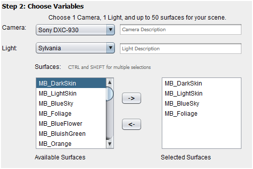
Because the user can only select 1 camera and 1 light for creating a .picture., I implemented the camera and light selection tools as combo boxes. These can display every camera or light in the dataset, but restrict the user to choosing 1 at a time. The surface selector, however, must enable the selection of up to 50 surfaces. Hence I used two lists . one for all possible selections, and one for currently selected surfaces . to make this possible. The user adds or removes surfaces to the selected surfaces list using the two arrow buttons.
Finally, part of the interaction was outputting the RGB data of the scenes the user generated. To display the textual RGB data, I used a simple text box. Together, these UI widgets allow the user to select 1 camera, 1 light, and up to 50 surfaces. We are now ready to let the user generate the RGB representation of the image given these variables.
Matrix operations: uncorrected color and ideal color
As described earlier, every light, camera, and surface is stored as a matrix. A surface is a 1D matrix (ie a vector) that has 1 row and n columns, where n is the number of data points it has (based on (end_wavelength . start_wavelength / interval). A camera is an nx3 matrix, where each column holds the sensor response for R, G, and B. A light is an nxn matrix where the diagonal is non-zero and stores the SPD data samples.
Additionally, there is an nx3 XYZ color matching function matrix (which can be thought of as the .ideal. camera) and a 3x3 sRGB matrix [6] which converts XYZ values to RGB for a standard monitor display.
Two RGB scenes are generated . one is the uncorrected version under the user-specified light and camera. The other is an .ideal. version that simulates a human observer under daylight, and serves as the example of what a color balancing algorithm should strive to achieve.
The uncorrected version is calculated as follows:
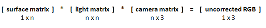
The ideal version is calculated as

Normalization
During the calculation of the RGB vectors, the matrices are normalized to 0 . 1 after multiplying by the camera matrix or the XYZ color matching function. The normalization is by the scale factor of the largest value in a scene. As an example, if there are 2 surfaces comprising a scene, with vectors [3, 4, 5] and [8, 9, 10], they are both normalized to 0-1 by dividing each by 10. After normalization, the values are converted to screen RGB values (for the ideal version, this happens after multiplication with the sRGB matrix) by multiplying by 255.
Results and Discussion
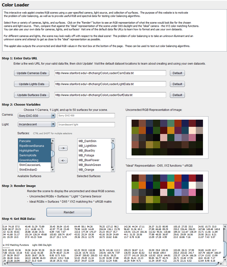
The end product . Color Loader . accomplished the objectives I had set out to fulfill. There are three sample datasets with 8 cameras, 42 lights, and 226 surfaces. These are loaded on startup as defaults. The user can access the raw spectral data by following the default links provided as part of the utility. Or, the user can upload their own data files, given that the files are on the same server and are properly formatted.
The interaction is intuitive, and is much faster than text files at letting the user see every camera, light, and surface in the dataset. The user can also display a scene for a selected light, camera, and up to 50 selected surfaces, and compare it against the ideal representation. This motivates color balancing, and provides data for color balancing algorithms to test against.
Practical Value
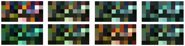
Comparing Lights
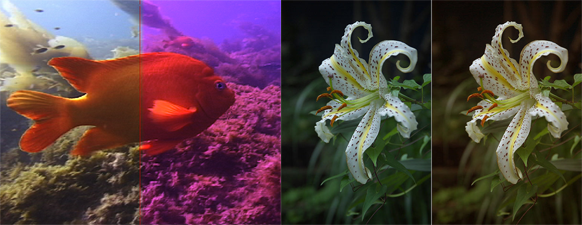
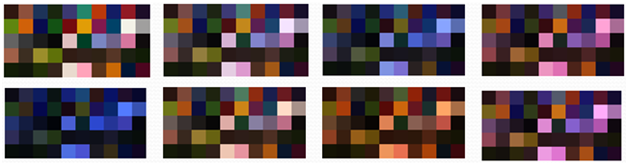
With Color Loader, the user can quickly visualize how changing illuminants will affect a scene. The following scenes have the same 50 surfaces, the same camera, but are illuminated with different lights. The top left scene is the .ideal. representation using D65 daylight and the XYZ matching functions.
Comparing Cameras
The same is possible with cameras. The following images have the same surfaces, the same illuminant, but are taken with different cameras. The top left is ideal.
Creating Scenes
An interesting application of Color Loader is the creation of custom scenes. Since each surface is named, and it is easy to quickly sort through the surfaces with the UI widgets, the user can group similar data to simulate a particular scene. The following are a couple examples:
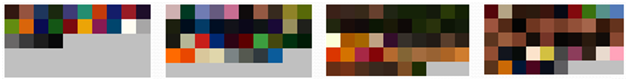
The leftmost scene contains the 24 MacBeth color checker patches. The next scene contains Dupont and Munsell paint chips. The third scene simulates a forest, with a collection of leaves, wood, bark, soil, and flowers. The last scene contains human skin reflectances and fabrics such as denim and cloth. Because some color balancing algorithms might handle certain scenes better than others, the flexibility to create custom scenes can help assess color balancing algorithms beyond the MacBeth color checker, and into more colorful scenarios.
Conclusion
An updated web database / color visualization utility has been presented, with added flexibility in terms of interaction, scene visualization, and custom scene generation. The Color Loader utility maintains the data transparency of static web databases currently available, while providing more functions that are conducive to exploration of cameras, lights, and surfaces, as well as how they interact. The resultant data motivates the issue of color balancing and can also aid in the testing of color balancing algorithm.
Future Work
1. Along with outputting RGB data, calculate the 3x3 matrix that would convert the uncorrected RGB to the ideal RGB.
2. Provide Gamma correction for display on different monitors.
3. Expand the default databases to contain more lights, cameras, and surfaces.
4. Allow plotting the raw spectral data of each light, camera, and surface.
5. Compatibility with Macintosh computers . rebuild using JDK 5, or wait until JDK 6 fixes its issues.
Acknowledgements
Many thanks to Dr. Joyce Farrell for her guidance throughout the project. Special thanks to Dr. Kobus Barnard for the data and clarifications.
References
[1] K. Barnard, .Synthetic Data for Computational Colour Constancy Experiments.. http://kobus.ca/research/data/colour_constancy_synthetic_test_data/index.html (views 3/19/2009)
[2] Spectra, NC State University Information Technology FTP server. ftp://ftp.eos.ncsu.edu/pub/eos/pub/spectra/ (viewed 3/19/2009)
[3] B. Smits. Spectral Data. http://www.cs.utah.edu/~bes/graphics/spectra/ (viewed 3/19/2009)
[4] K. Barnard, L. Martin, B. Funt, and A. Coath, " Data for Colour Research," Color Research and Application, Volume 27, Issue 3, pp. 148-152, 2000.
[5] ImageEval Consulting, LLC. http://www.imageval.com/public/index.htm (viewed 3/19/2009)
[6] Specification of sRGB (in IEC 61966-2-1:1999). http://www.color.org/sRGB.pdf (viewed 3/19/2009)
Appendix
Presentation (PDF)
Try it out! (Color Loader)
Source Code Bundle (RAR)
Spectral Data (CamData LightData LightData2 Surfaces XYZData)