The engineering prototype came with an encoder script, disp14enc, which takes in an HDR-format image and outputs a bitmap file (.bmp) which can then be placed into the graphics card framebuffer (The simplest way to do this is to simply load the bitmap and make it appear full-screen). The encoder is written in the CSH shell scripting language, and uses many utility tools from the Radiance raytracer distribution. The script source can be found in the "Source code and data" section.
The script chains together many simple manipulations of the source image, most of which map fairly directly to Matlab image processing toolbox equivalents. These include common operations such as image resizing and filtering, and slightly less common operations such as convolution, and luminance conversion. The difficult part of the conversion was in simply understanding the original script and the functioning of the many utility programs it calls upon. Below is a flowchart of the encoding script.

First, the script resizes and possibly crops the source image to fit the resolution of the display. The result of this represents the ideal luminance output image that the encoder will attempt to reproduce
To calculate the LED backlight drive values, the script follows a multi-step algorithm. First, the ideal image is converted to luminance space and color information is discarded. A gamma curve is applied, perhaps to scale down the input dynamic range to some extent. Then, the luminance image is downsampled to a size of (33,46) using a combination of box and gaussian filtering to avoid aliasing. The LED backlight grid is a hexagonal arrangement with 46 rows of 17 or 16 LEDs per row. Filling in this hex grid to make it rectangular results in a grid of size (33,46). Therefore, the downsampled luminance image represents the 'ideal' backlight distribution over a rectangular grid.
In the display, each LED has a very wide point-spread function (PSF). That is, turning on a single LED creates a very broad illumination pattern reaching across most of the screen. Therefore, the values in the ideal backlight image cannot be directly used as LED drive values, as the luminance at an LED is influenced strongly by the luminance of neighboring LEDs. Therefore, a simple cross-talk model is used by the script to reduce the drive strengths of LEDs to account for this cross-talk. After that, the image pixels that actually correspond to LED locations are extracted and normalized. Since the LEDs do not have a linear response curve, the inverse of that curve is used to find the framebuffer values that correspond to the calculated drive values.
Since the illumination pattern created by the LEDs is low-frequency, the LCD front panel has to both include the high-frequency modulation (and all the color) of the source image, and compensate for the unwanted low-frequency content possibly introduced by the backlight. First, therefore, the per-pixel backlight luminance must be calculated. This is done by taking the hex-grid pattern of the LED drive values, and filtering it with the PSF of the LEDs. The PSF is approximated as a sum of two gaussians (one narrow and peaked, one wide and flat), and therefore the backlight image can be easily calculated by gaussian filtering followed by upscaling.
With the full-resolution (normalized) backlight image, calculating the LCD values is straightforward. The ideal input image values are simply divided by the backlight luminance values to create the LCD drive values, with appropriate normalizations and handling of division-by-zero. The LCD values are then compensated to account for the tint of the LEDs (which seem to have a slight yellow tint), and the inverse of the LCD response curve is applied to generate the final LCD framebuffer values.
The final step of the algorithm correctly places the LED drive values on row 2 of the framebuffer image. The mapping of LEDs to pixels is a complex one, with gaps in the pattern, but the LED drive values all end up between pixels 3 and 1002, inclusive, on row 2 of the image.
There are several other details involving exposure levels, processing multiple animation frames in a row, and so on, but the above covers the important details.
To match the output of disp14enc, several of the parameters duplicated from the script had to be tweaked. This is likely due to differences in algorithm implementation, and differing definitions for widths of filters. For example, the radii for various gaussian filtering steps typically had to be multiplied by a factor of 0.75 to achieve equivalent output images. Therefore, hdrEnc(the Matlab port) and disp14enc do not produce pixel-identical output. However, the differences between the two are very small as can be seen in "Matlab port comparison"
While the basic BrightSide-supplied encoder is fast, it is not terribly accurate. It implements a very simple crosstalk analysis in order to find LED values that would create a backlight image close to the ideal, as represented by the downsampled luminance image. Therefore, attempting to improve this step of the encoding process seemed like a natural idea.
The mapping of LED brightness values to the resulting backlight image is linear - doubling LED intensity will double its contribution to the backlight image. This means the map can be represented by a matrix, and the mapping by multiplying a vector of LED drive values by this map. This will output a vectorized form of the backlight image, which can then be rearranged into a normal 2D image.
Given an ideal backlight image, then, the relationship between the LED drive values and the backlight image can be described by the following linear equation:
Here, we know i and M, and want to find d. Assuming we are solving the problem at the resolution of the rectangular LED grid, i will be a vector of length 33 x 46 = 1518, and d has a length of 759, the number of LEDs. Therefore, M is a rectangular matrix of dimensions (1518,759), and we cannot directly invert M.
However, this is a typical situation for using a least-squares solution, especially since we know that we likely cannot match most ideal backlight images exactly, but only to a limited degree. Least-squares will find a vector d that minimizes the mean-square error
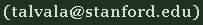
A least-squares solver is built into Matlab. However, attempting to use it results in the following values for d for the Memorial Church scene:
The least-squares solution requires negative drive values for many LEDs, which is of course a physical impossibility. Clearly, the naive least-squares solution is infeasible. (Note that the original crosstalk algorithm can also result in negative values - those are clamped to zero after the crosstalk calculation is complete)
However, the least-squares error metric is a reasonable one to adopt. In general, lower mean-square error means lower perceptible differences between the result and the ideal image, even though mean-square error does not take into account that errors are more acceptable in certain image regions than in others.
What seems reasonable, then, is to still use a least-squares error metric, but somehow add in the additional constraint that the resulting d vector should have all positive entries. The CVX convex optimization Matlab toolbox was chosen for this task. CVX is a front-end to a convex optimization solver called SeDuMi, and makes it easy to specify and solve a given constrained problem. The abilities of the solver extend far beyond what is needed to solve the simple objective function and constraint that are needed for this project, but its user-friendliness made it an appropriate choice. The following lines contain the entirety of the Matlab code used to call CVX and solve the optimization problem:
Besides replacing the crosstalk correction with the above minimization, with the convex optimizer version of the encoder, creating the full-resolution backlight image is different. Since matrix M is known, the backlight distribution is just an unscaled version of M*d. Besides other small changes to account for normalization factors, the rest of the encoder is as before. Below is block diagram of the convex optimizer version:

Since the optimization problem is solved at low resolution, the question of whether the low-resolution solution is equivalent to solving at full resolution (which is intractable due to the sheer size of the mapping matrix). Given that the PSF of the LEDs is well-approximated by gaussians, which are very well-behaved when downsampled, it seems unlikely that the low-resolution optimization would introduce noticeable error into the procedure. However, this has not been confirmed experimentally.
Finally, there is the question of how to produce the mapping matrix M. For this, and for performing quantitative comparisons of encoder output, the HDR simulator was written. It is described in the next section
When writing an encoder for any system, is it important to be able to validate its functioning as well as quantify its performance. While the BrightSide HDR display itself could be used for validation, it cannot easily be used for quantifying encoder performance, especially outside of subjective image similarity comparisons. And during development of an algorithm, requiring constant access to the HDR display can become cumbersome. For those reasons, the HDR display simulator was written. By default, it uses analytic approximations to the display parameters used by disp14enc, but it can be given alternate values for such parameters as LED/LCD response curves, LED PSFs, and the LED positions.
The simulator reads in an encoded framebuffer, such as the ones created by disp14enc or hdrEnc, described above. It then extracts the LED drive values, and uses the LED response curve to map frame buffer values to actual drive values. It creates a point-light version of the backlight by placing LED values in the right places on the hexagonal backlight grid. The point-source image is then convolved with the LED PSF to create the actual backlight luminance pattern. Finally, tinting factors are used to weight the output color of the LEDs slightly to the yellow.
Like the LED values, the LCD image is mapped through the LCD response curve. Notably, the minimum possible value for LCD output is 0.52, and the maximum is 217.7, giving a maximum contrast ratio of 418:1, which is the also the maximum local contrast ratio for the display.
Then, the LED backlight image is multiplied together with the LCD panel image to create the final output luminance pattern. It is then normalized to the empirically measured output brightness of the display, so that the display with only one lit LED and set to 150 (framebuffer value), and with the LCD set to 255 gives an output luminance of 256 cd/m^2.
For quantitative comparisons of encoders, the simulator can be used to generate the actual resulting luminance pattern on the display, which can be compared to the input HDR image. This requires normalizing the images to some common measure, since the simulator outputs physically meaningful units, and the input HDR images are typically not in any particular unit.
The simulator was also used to generate the mapping matrix M for the convex optimizer. As the matrix describes how each LED drive value maps to the complete backlight light distribution, it can be synthesized with one call to the simulator per LED. For each call, the LCD is set to fully transmissive, and only one LED is turned on. The simulator output image is then downsampled to fit the ideal backlight image dimensions, and then converted to a vector that represents a single row of the M matrix. Generating the matrix is time-consuming, taking roughly 30 minutes, so it is precalculated and simply loaded by the encoder when needed.
The simulator is intended to be flexible to allow better measurements of the display's parameters to be plugged in once they become available, and the script to regenerate the mapping matrix is also included with it to allow M to be recalculated to be more accurate.