Result
Following are some demosaicing results:
1. Point Array (With good optics setting)
 |
 |
 |
 |
 |
 |
| Origin |
Bilinear Interpolation |
Two Line Interpolation |
Data Dependent Triangulation |
Edge Directed Interpolation |
High Quality Linear Interpolation |
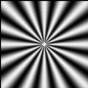
2. Point Array (With Poor optics setting)
 |
 |
 |
 |
 |
 |
| Origin |
Bilinear Interpolation |
Two Line Interpolation |
Data Dependent Triangulation |
Edge Directed Interpolation |
High Quality Linear Interpolation |
In the point array pattern, high quality linear interpolation (HQL) is much better than others.
This is because HQL uses the information of all three channels to estimate the missing color pixels,
and in such a gray level image RGB channels are highly correlated to each other.
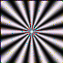
3. Mackay Pattern (With Good optics setting)
 |
 |
 |
 |
 |
 |
| Origin |
Bilinear Interpolation |
Two Line Interpolation |
Data Dependent Triangulation |
Edge Directed Interpolation |
High Quality Linear Interpolation |
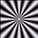
4. Mackay Pattern (With Good optics setting but with some noise)
 |
 |
 |
 |
 |
 |
| Origin |
Bilinear Interpolation |
Two Line Interpolation |
Data Dependent Triangulation |
Edge Directed Interpolation |
High Quality Linear Interpolation |
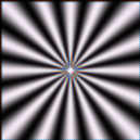
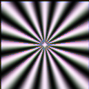
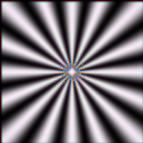
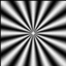
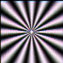
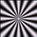
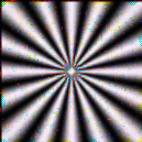
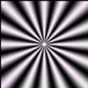
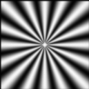
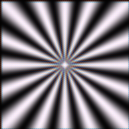
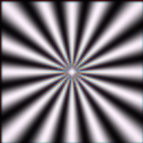
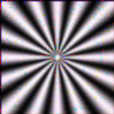
5. Mackay Pattern (With Poor optics setting)
 |
 |
 |
 |
 |
 |
| Origin |
Bilinear Interpolation |
Two Line Interpolation |
Data Dependent Triangulation |
Edge Directed Interpolation |
High Quality Linear Interpolation |
Now we can see some difference between each algorithm. HQL still gives a better result in gray
image. Two-line interpolation (TL) now has some notible noisy spot in its result. It's interesting
that edge-directed interpolation (ED) also has some noisy spots. It is because in the core of ED's
algorithm it requires an inverse matrix which may not exist. In that case matlab will return a poor
approximation of the inverse matrix. I believe this is the main reason of these obvious noisy spots.
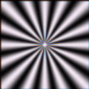
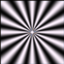
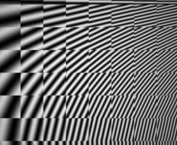
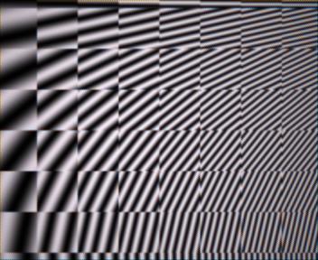
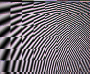
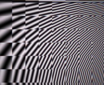
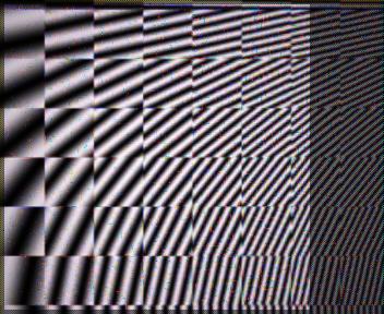
6. Frequecy Orientation Pattern
 |
 |
 |
 |
 |
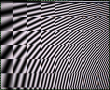 |
| Origin |
Bilinear Interpolation |
Two Line Interpolation |
Data Dependent Triangulation |
Edge Directed Interpolation |
High Quality Linear Interpolation |
For color images, click on the image to see a large (512x512) one.
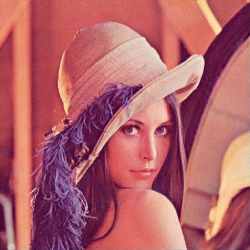
7. Lenna
 |
 |
 |
 |
 |
 |
| Origin |
Bilinear Interpolation |
Two Line Interpolation |
Data Dependent Triangulation |
Edge Directed Interpolation |
High Quality Linear Interpolation |
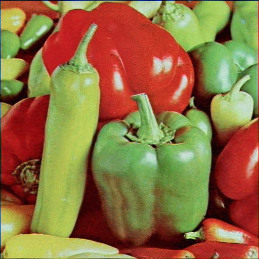
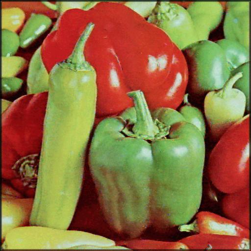
8. Peppers
 |
 |
 |
 |
 |
 |
| Origin |
Bilinear Interpolation |
Two Line Interpolation |
Data Dependent Triangulation |
Edge Directed Interpolation |
High Quality Linear Interpolation |
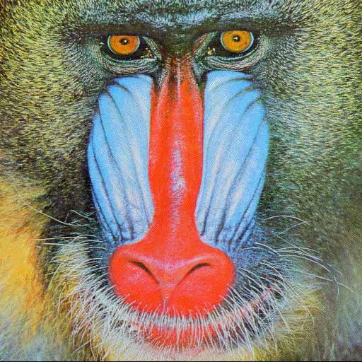
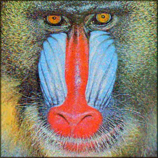
9. Baboon
 |
 |
 |
 |
 |
 |
| Origin |
Bilinear Interpolation |
Two Line Interpolation |
Data Dependent Triangulation |
Edge Directed Interpolation |
High Quality Linear Interpolation |
PSNR
| | Bilinear | Two Line | DDT | ED | HQL |
| pointArrayGoodOptics | 36.3648 | 35.7747 | 35.6585 | 35.4222 | 41.1929 |
| pointArrayPoorOptics | 36.9486 | 35.5251 | 36.0582 | 35.9671 | 43.3026 |
| Mackay-GoodOptics | 35.1965 | 30.3028 | 34.5957 | 30.4705 | 39.0364 |
| Mackay-GoodOptics-Noisy | 34.4876 | 30.0661 | 33.9442 | 28.8066 | 38.6460 |
| Mackay-PoorOptics | 36.6779 | 31.0248 | 36.0480 | 30.8752 | 39.8976 |
| FREQ-ORIENT | 25.6803 | 20.7551 | 24.3690 | 15.0310 | 23.4313 |
| Lenna | 29.0966 | 26.7559 | 29.5427 | 21.3632 | 23.8906 |
| peppers | 28.5986 | 25.2555 | 27.1646 | 22.2679 | 25.7284 |
| babbon | 21.1712 | 19.6614 | 20.7621 | 17.3188 | 20.8455 |
< Algorithm > < Conclusion >
< Home >