Algorithm Description
In this section we introduce four prevailing demosaicing algorithms:
- Pixel-Value Data-Dependent Triangulation
- Two Line Interpolation
- Edge Directed Demosaicing
- High Quality Linear Interpolation
Pixel-Value Data-Dependent Triangulation (DDT)
It is known that the human visual system makes significant use of edges. To take the advantage of
this fact, a new edge-directed method is introduced. Consider the case that there is an edge passing
between a square of four pixels. If this edge cuts off one corner, one pixel will be substantially
different to the other three, as shown in Fig. 2.

Figure 2: Triangulation in a four-pixel square
We call this pixel the outlier. As a result, for each square of four pixels, if pixel d is
an outlier, it may imply an edge passing along the diagonal (a,c). In effect, the three similar
pixels define a plateau, and this gives us a hint that if we want to interpolate a higher resolution
pixel within the relatively flat region we should not use the outlier. Classical interpolation
methods suffer from edge blurring because they use all four pixels to do interpolation, while DDT
uses only three.
To implement this algorithm, we follow these two steps:
- For each square of four pixels {a,b,c,d}:
- For each pixel to be interpolated:
- Find the triangle where the pixel is
- Linear interpolate the pixel by the vertices of the triangle.
Two Line Interpolation
Most of the interpolation methods look for best recovery quality, and therefore some of them might
not be feasible to low-cost comsumer products due to their high computational complexity and high
memory usage. This algorithm introduces a way to interpolate high resolution image by using only one
image line buffer.
 Figure 3:(a)Pixel prediction at x using
three neighboring pixels.
Figure 3:(a)Pixel prediction at x using
three neighboring pixels.
(b)Interpolation at x using a two-line buffered neighborhood
We will use following function for computing the value at x:
 | (1) |
where
 | (2) |
There are four differnt neighborhood combinations, which is shown in Fig. 4.
 Figure 4: Four different neighborhood combinations.
For green pixel interpolation (See Fig. 4(a), 4(b) ), we use following equation:
 | (3) |
For red pixel interpolation, consider the following three cases:
CASE 1: (See Fig. 4(c) )
Let 
If(  )
)
else
CASE 2: (See Fig. 4(d) )
Let 
If(  )
else
)
else
CASE 3: (See Fig. 4(b) )
Let 
If(  )
else
)
else
For blue pixel interpolation, computations are similar to
the red interpolation cases.
Edge Directed Demosaicing
This algorithm introduces the local covariance to the recovery of the missing color pixels. First we
interpolate the interlacing lattice  from
from
 . We constrain ourselves to the fourth-order linear interpolation
(refer to Fig. 5)
. We constrain ourselves to the fourth-order linear interpolation
(refer to Fig. 5)
 | (4) |
According to classical Wiener filtering theory [7], the optimal MMSE linear interpolation
coefficients are given by
 | (5) |
where  and
and  are the
local covariances at the high resolution.
are the
local covariances at the high resolution.
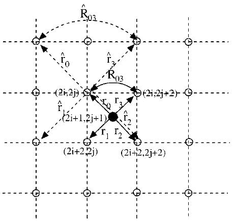 Figure 5: Geometric duality when interpolating
from
Figure 5: Geometric duality when interpolating
from
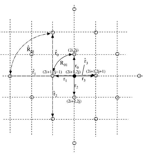 Figure 6: Geometric duality when interpolating
 (i+j = odd) from (i+j = even)
To approximate  , we use the low-resolution covariances:
 | (6) |
where  is the data vector containing the MxM pixels inside
the local window and C is a 4xM^2 data matrix whose th column vector is the four nearest neighbors
of y_k along the diagonal direction. By (5) and (6) we have:
is the data vector containing the MxM pixels inside
the local window and C is a 4xM^2 data matrix whose th column vector is the four nearest neighbors
of y_k along the diagonal direction. By (5) and (6) we have:
 | (7) |
The edge-directed property of covariance-based adaptation comes from its ability to tune the
interpolation coefficients to match an arbitrarily-oriented step edge. However, the principal
drawback with covariance-based adaptive interpolation is its prohibitive computational complexity.
For example, when the size of the local windowis chosen to be M=8, the computation of (6) requires
about 1300 multiplications per pixel. A compromised solution is applying this method only to the
edge pixels and using bilinear interpolation for the non-edge pixels. A pixel is declared to be an
edge pixel if the local variance estimated from the nearest four neighbors) is above a preselected
threshold.
High-Quality Linear Interpolation
Classical bilinear interpolation methods use only the color information in the channel to be
interpolated. For example, when a green pixel is to be estimated, classical methods usually use only
information in the green channl. In this high-quality linear interpolation method it combines
bilinear interpolation with a gradient-correction gain and turns out a better estimation of the
missing color informaiton.
Specifically, to interpolate G values at an R location, we use the formula:
 | (8) |
where  is the biliear interpolation and
  is the gradient of R computed by:
 | (9) |
In addition to the interpolation and gradient, we also use gain parameter {Ł\,Ł],Ł^} as the gain
factor in R,G,B channel, respectively. Empirically they are Ł\=1/2, Ł]=5/8, and Ł^=3/4. After
applying these gain factor to the gradient-correction part, we can compute the equivalent FIR filter
coefficient for each interpolation case. The result coefficients are shown in Fig. 7.
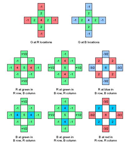
Figure 7: Filter coefficients for the proposed linear
demosaicing method
< Introduction > < Result >
< Home >