Read noise

1)     Background

Read noise is a property that is inherent to the CCD of digital cameras, and is present in all images taken and recorded by a camera. The read noise of a camera affects how well the image represents the actual data, since high read noise decreases the quality of the image. Calibrating the read noise allows us know more about the quality of the CCD as well as the data distortion due to the reading of images.

2)     Methods

The read noise calculation requires values of a pixel taken over a time series. For this calibration, we took pictures in the Nikon raw format with the lens cap on. 100 pictures were taken at each of eight exposures: 1s, 2s, 4s, 8s, 15s, 20s, 25s and 30s, in order to obtain the pixel values over a time series. Averaging the pixel values over time will then give us the read noise.

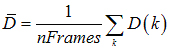
The calculation is as follows:

                                                              i.      Average the values of a single pixel over the 100 photos taken

                                                            ii.      Subtract this average value from the original images

                                                          iii.      Obtain the temporal variance of the pixel values

                                                           iv.      Repeat the calculations for different exposure values to compare the read noise values obtained.

Theoretically, the read noise should remain constant across all pixels in the camera, and we could obtain the read noise using just the data of a single pixel over a time series. However, because of variations in conditions such as temperature and in the manufacturing process, we expect small differences in the read noise values obtained for different pixels. In addition, we expect more significant differences in the read noise values obtained for pixels of different colored-sensors. We used Matlab to analyze our data and results.

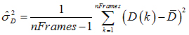
As there are more than 6 million pixels in every image, it will be extremely time-consuming to compute and compare the read noise values obtained for each different pixel in the image. An accurate estimation of the read noise can be obtained by taking a sample of these 6 million pixels. For our methods, we decided to compute the read noise for 400 pixels, evenly spaced along a diagonal of the image, since this will allow us to analyze the variation of read noise across the entire image instead of only in a small region. The pixels sampled can be visualized as such:

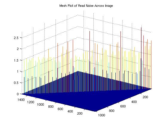
Figure 1: Image showing the pixels sampled across the image

3)     Results

The figures below show the variances in the read noise for pixels across the width of the image (1520 pixels) for each of the eight exposure values that we analyzed. The top figure shows the variances in the read noise for the different sensors (green, blue and red) on the CCD for each exposure time, with the color of the line corresponding to the color detected by the sensor. The figure on the right plots the read noise across the image for different exposure times on the same axes.

From the graphs, we can see that for short exposure times, the read noise remains generally constant across the image at around 10 to 20. However, for exposure times 8s and greater, the read noise starts at around 50 for pixels close to the edge of the image, before falling off to values around 20 for pixel positions after 500. We postulate that this is due to the order that the camera reads in the images. The higher read noise at lower pixel positions can be explained if the camera reads in the image starting from the highest pixel values. Since the lower pixel values are read in last, their values are more likely to be changed before they are read in and stored by the camera, leading to higher noise.

Figure 2: Graphs of read noise across the image for different color channels at different exposures

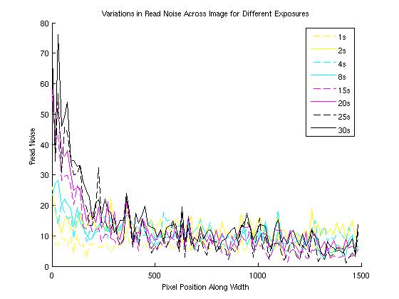
Figure 3: Graph of variation in read noise across different exposure times

We then compare the variances of the read noise across different exposure times by averaging the read noise for each exposure for each channel (red, blue and green). This analysis will enable us to find out how the reads noise for each color channel varies across exposure times, as well as how they vary relative to one another. The graph is plotted below.

From the graph, we can see that the read noise increases with increasing exposure time for all three color channels. On average, the blue sensors produce the greatest read noise, followed by green and then red sensors.  The lowest average read noise is around 7 pixels for the red channel at 1s exposure, and the greatest is 16.5 from the blue channel at 30s exposure.

Plotting the 2 green channels separately, however, produces different results. The solid green line in the figure is the average of the 2 green sensors present per image point, and the actual read noise for each of the two green sensors is plotted as dashed green lines in the figure. We observe that one of the green channels consistently has higher noise than all the other channels, and this explains the green spikes we see in figure 2, where we plotted the read noise across pixels for each channel.

The black line gives the read noise averaged across all pixels for all color channels at each exposure, and these values can be used for our simulation in ISET.

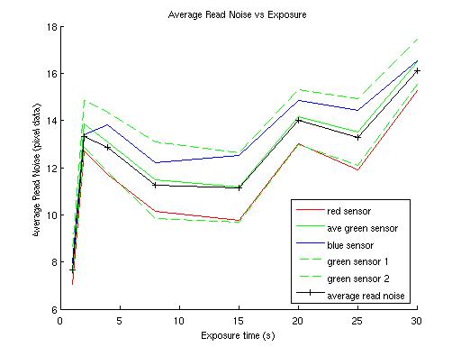
Figure 4: Average read noise

From our analysis, we found that the read noise is not constant across all pixels in the image. It varies depending on the pixel location, the color that the pixel senses as well as the exposure time. Of all these three factors, the read noise increases most with increasing exposure time, hence we would expect a greater difference between the original data and the image for higher exposure times.

Next: Spectral Response Function | Home