Macbeth Color Checker

    Analysis and Predictions

1)     Actual Performance Results

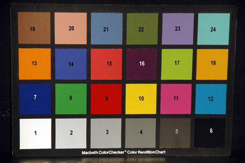
Figure 1. Numbered Macbeth Color Checker for reference

The following two figures summarize the data obtained from the raw .NEF files of the color checker in tungsten light.

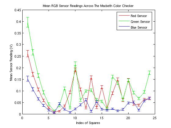
Figure 2. Mean RGB Sensor Readings Across the Macbeth Color Checker.

This figure shows the mean RGB sensor readings across the squares of the Macbeth Color checker, as well as the standard deviations which are represented by the error bars. For instance, the first six squares of the checker go from white to black, and can be clearly seen in the graph to have decreasing sensor readings for all three sensors. The largest response in these first six square comes from the green sensor, which is what we expected having found that the spectral response function was the largest for green.

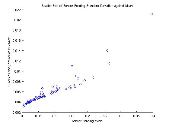
Figure 3. Scatter Plot of Sensor Reading Standard Deviation Against Mean.

This scatter plot of the standard deviations against the mean values illustrates the general trend in the raw data of noise increasing with the light intensity falling on the sensor. This is a result of photon noise as well as PRNU.

The data obtained from the JPEG images taken in tungsten light are shown in the two figures below.

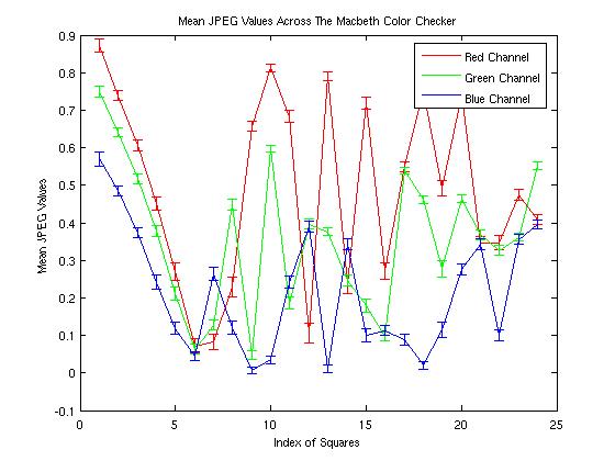
Figure 4. Mean JPEG Values Across the Macbeth Color Checker.

Looking at the first six data points which correspond to the six bottom squares of the color checker that run from white to black, compared to the data obtained from the raw images, it can be seen that the green channel no longer shows the largest values. We hence infer that the camera’s processing pipeline adjusts the gains for the different channels between the raw data and JPEG file, compensating for the larger green sensor sensitivity that we observed in the spectral response function.

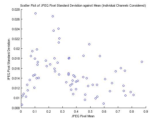
Figure 5. Scatter Plot of JPEG Pixel Standard Deviation against Mean.

This scatter plot of the standard deviation against mean values for the JPEG image no longer shows the same correlation of increasing noise with intensity that was observed in the raw image. This is most likely due to both the adjustment of the gains in the different channels, as well as the JPEG compression process.

The following 4 graphs were generated from the raw and JPEG data for the color checker in blue-filtered tungsten light. With the blue filter, the light incident on the Macbeth Color Checker and subsequently reflected has a relatively large blue component, and this makes the blue response now much more significant despite the relatively smaller blue sensor spectral response.

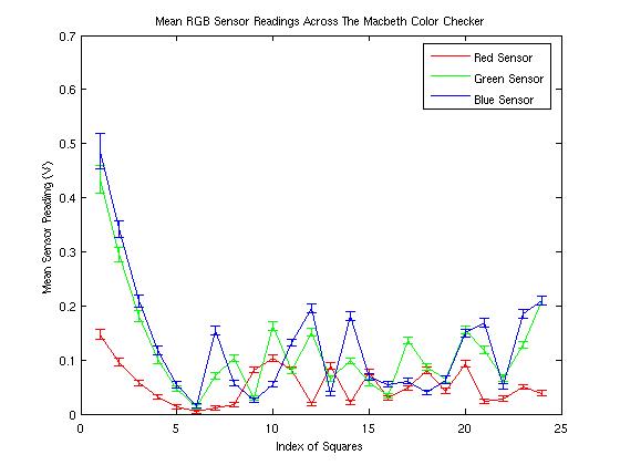
Figure 6. Mean RGB Sensor Readings Across Macbeth Color Checker (Blue Light).

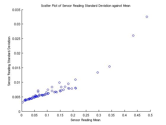
Figure 7.. Scatter Plot of Sensor Standard Deviation Against Mean (Blue Light).

The graphs for the JPEG data once again illustrates the processing done by the camera between the raw and JPEG files where different gains are used for the red, green and blue channels.

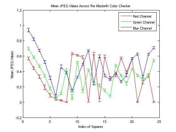
Figure 8. Mean JPEG Values Across the Macbeth Color Checker (Blue Light).

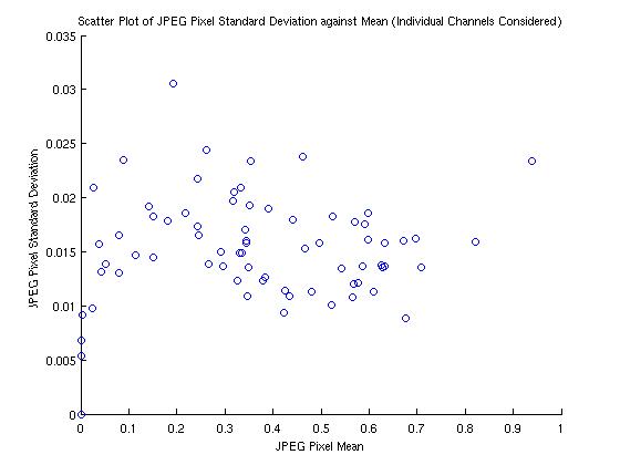
Figure 9. Scatter Plot of JPEG Pixel Standard Deviation against Mean (Blue Light).

5)     Predictions

We opted to directly predict the RGB values for the Macbeth Color Checker squares to evaluate the accuracy of our estimated sensor spectral responses. Using the reflectance readings taken with the spectroradiometer for each of the squares, we multiplied it by the spectral response matrix to obtain predicted RGB values for all 24 squares in the two lighting conditions.

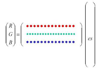
Figure 10. Matrix Multiplication With Spectral Response Function

We assumed that our predicted RGB values would differ from the RGB values of our image data by an approximately linear scaling factor. This linear scaling factor comes from the difference in the length of exposure between the initial calibration and the photographing of the Macbeth Color Checker. In addition, the lens of the camera was removed in the initial calibration exercise, but was used in the photographing of the Color Checker. Although the effect of the lens may not be a simple linear scaling of the intensities across all wavelengths, it will be approximated as one for our purposes. We therefore fit the values to a linear function to find the approximate scaling and used it to normalize the predicted values.

Tungsten Lighting

The graphs below show a comparison of the actual measured raw mean pixel values for the three channels and the predicted raw mean pixel values.

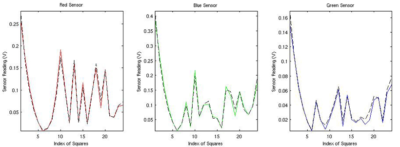
Figure 11. Measured and Predicted RGB Values for Macbeth Color Checker in Tungsten Light. The colored lines represent the measured values while the black dashed lines are the predicted values.

Figure 12 . Mean Squared Error for RGB Channels in Tungsten Light.

On the whole, our spectral response functions did very well in predicting the RGB values of the squares. The mean squared error was on the order of 0.1% of the mean intensity in all three of the channels. This shows that the relatively simple linear systems approximation method worked well.

Tungsten Lighting with Blue Filter

The graphs below show a comparison of the actual measured raw mean pixel values for the three channels and the predicted raw mean pixel values.

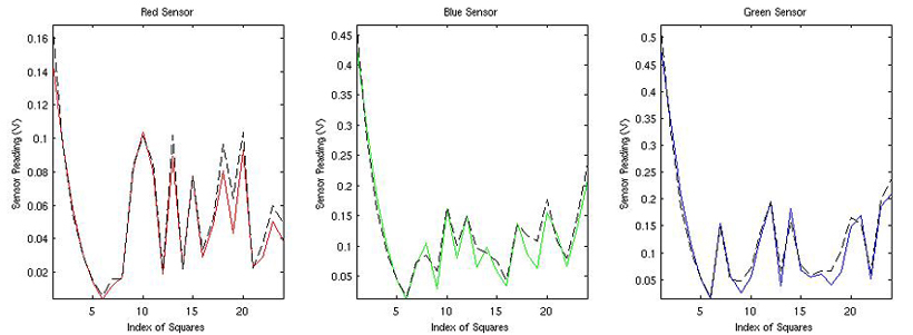
Figure 13. Measured and Predicted RGB Values for Macbeth Color Checker in Tungsten Light with Blue Filter. The colored lines represent the measured values while the black dashed lines are the predicted values.

Figure 14. Mean Squared Error for RGB Channels in Tungsten Light for Blue Filter.

Similarly, our spectral response functions did well in predicting the RGB values of the squares even with the blue filter. The mean squared error was still on the order of 0.1% of the mean intensity in all three of the channels.

Next: Conclusion | Home