GRADIENT-BASED DYNAMIC RANGE COMPRESSION
RESULTS
|
The algorithm performed quite efficiently, given the fact that it is running on MATLAB: for
a 768x1024 image, the algorithm took roughly a minute to complete on the computers in the
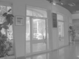
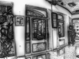
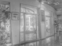
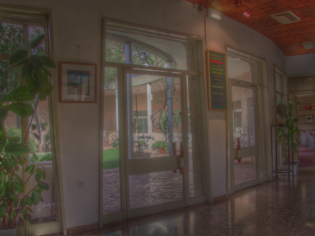
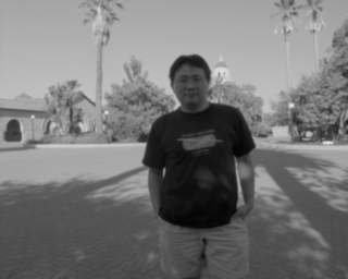
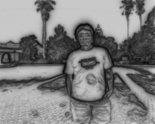
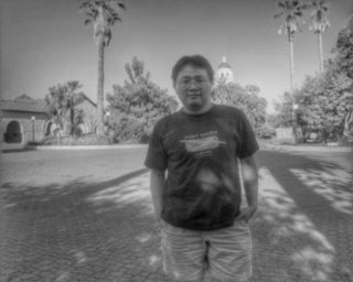
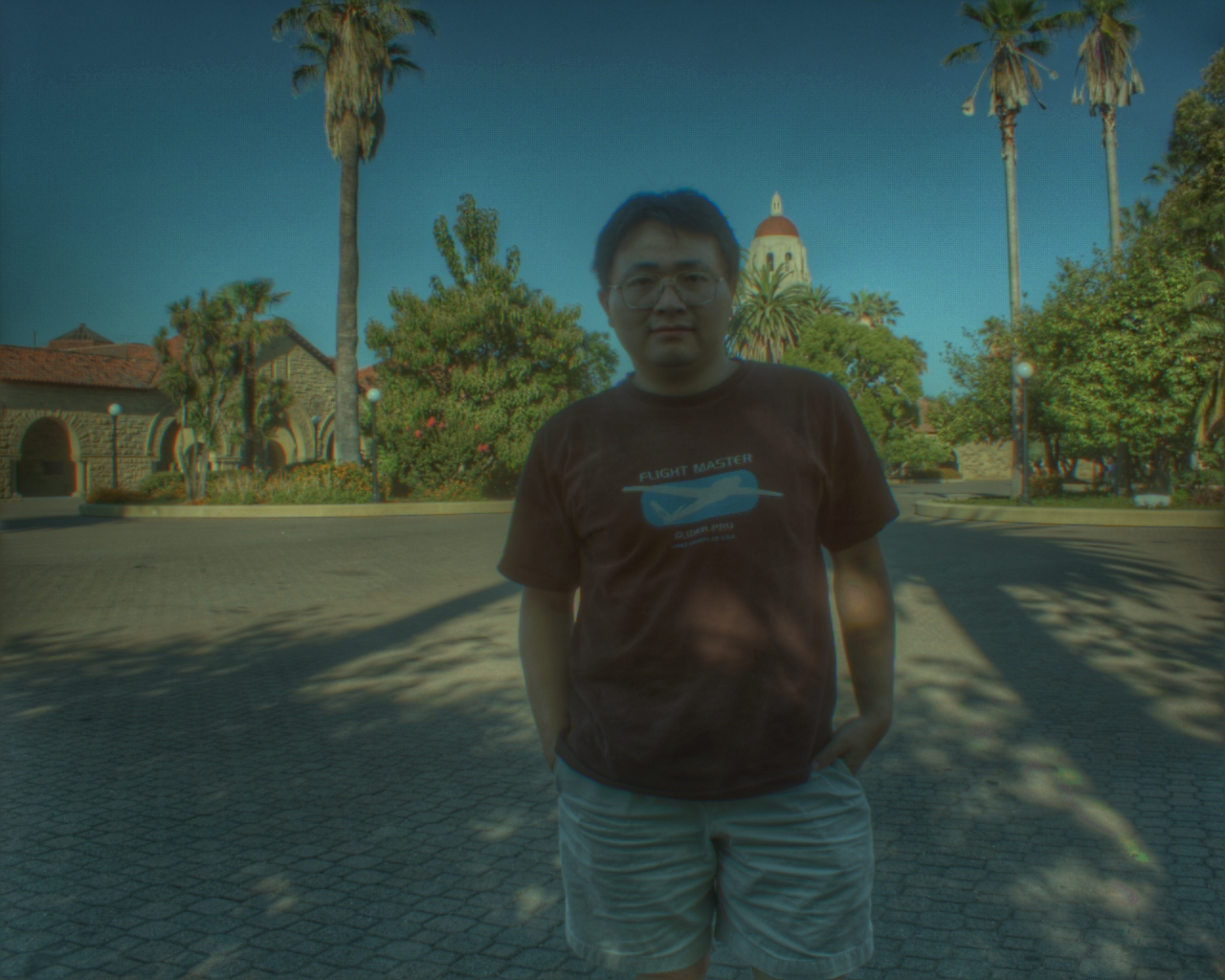
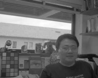
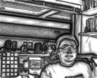
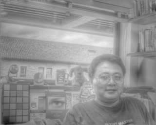
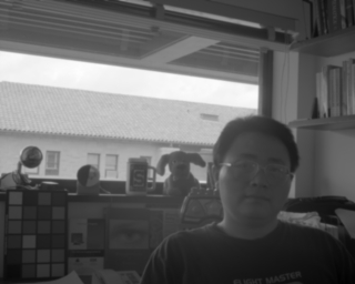
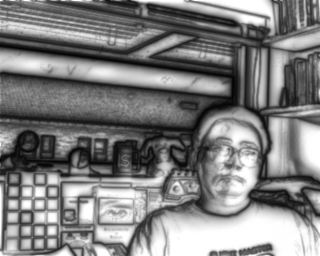
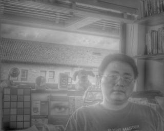
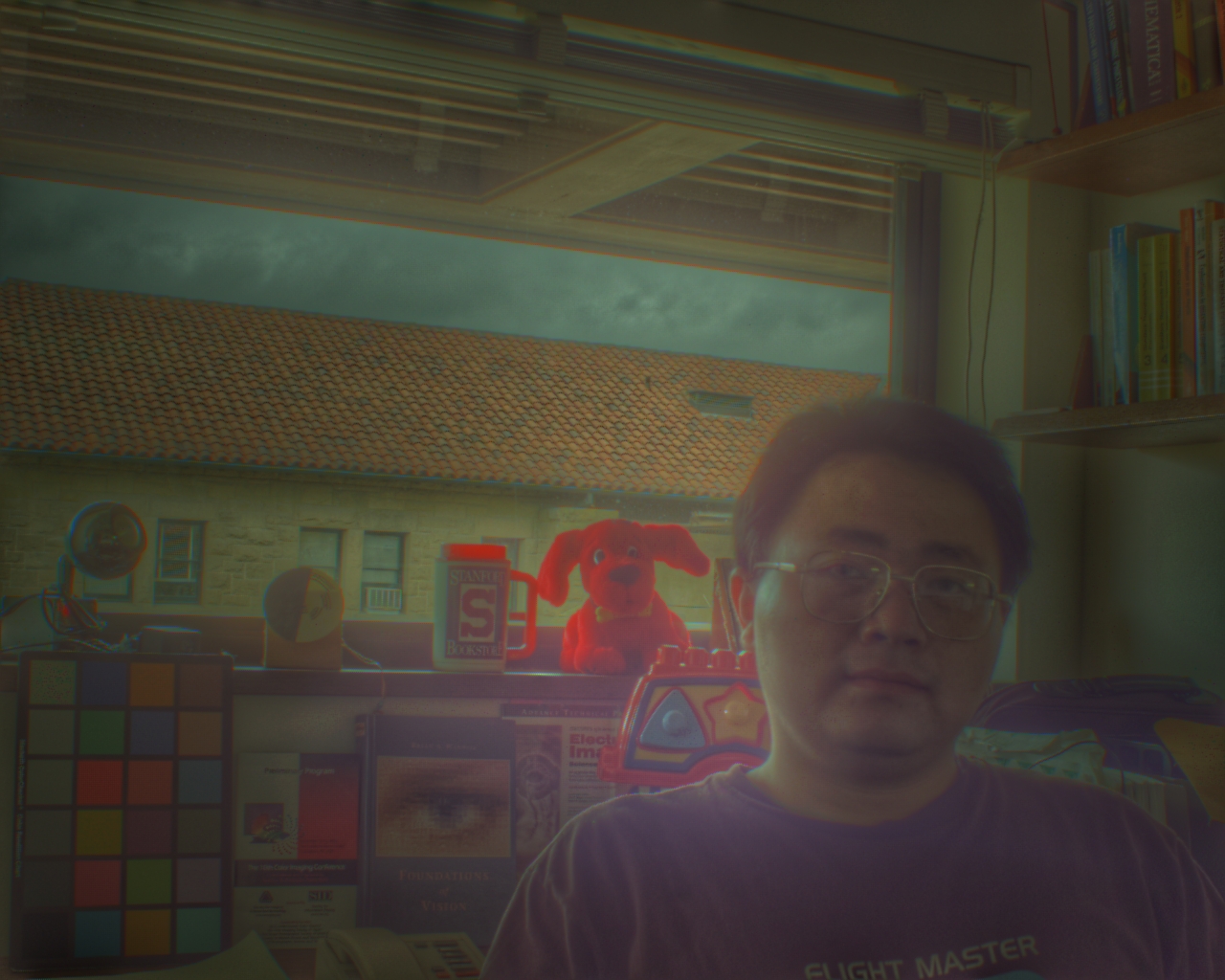
Stanford ISE lab. Below are a number of images illustrating the progression of the algorithm and the final result. Four subimages are shown for each picture we ran the algorithm on: the original logarithmic intensity image (top left), the gradient attenuation function (top right), the final logarithmic intensity image (bottom right), and the final color output picture. Note that all the images were originally at 1280*1024 (except for the belgium picture, which was slightly smaller than the rest at 768*1024). |
The Belgium image went from a dynamic range of 5.79 to 1.08 log units, using alpha = 0.3, beta = 0.85, and s = 0.6.
 |
 |
 |
 |
The SunShadePerson image went from a dynamic range of 2.67 to 0.73 log units, using alpha = 0.3, beta = 0.9, and s = 0.6.
 |
 |
 |
 |
The OfficeLightsOnPerson image went from a dynamic range of 3.65 to 0.67 log units, using alpha = 0.2, beta = 0.85, and s = 0.6.
 |
 |
 |
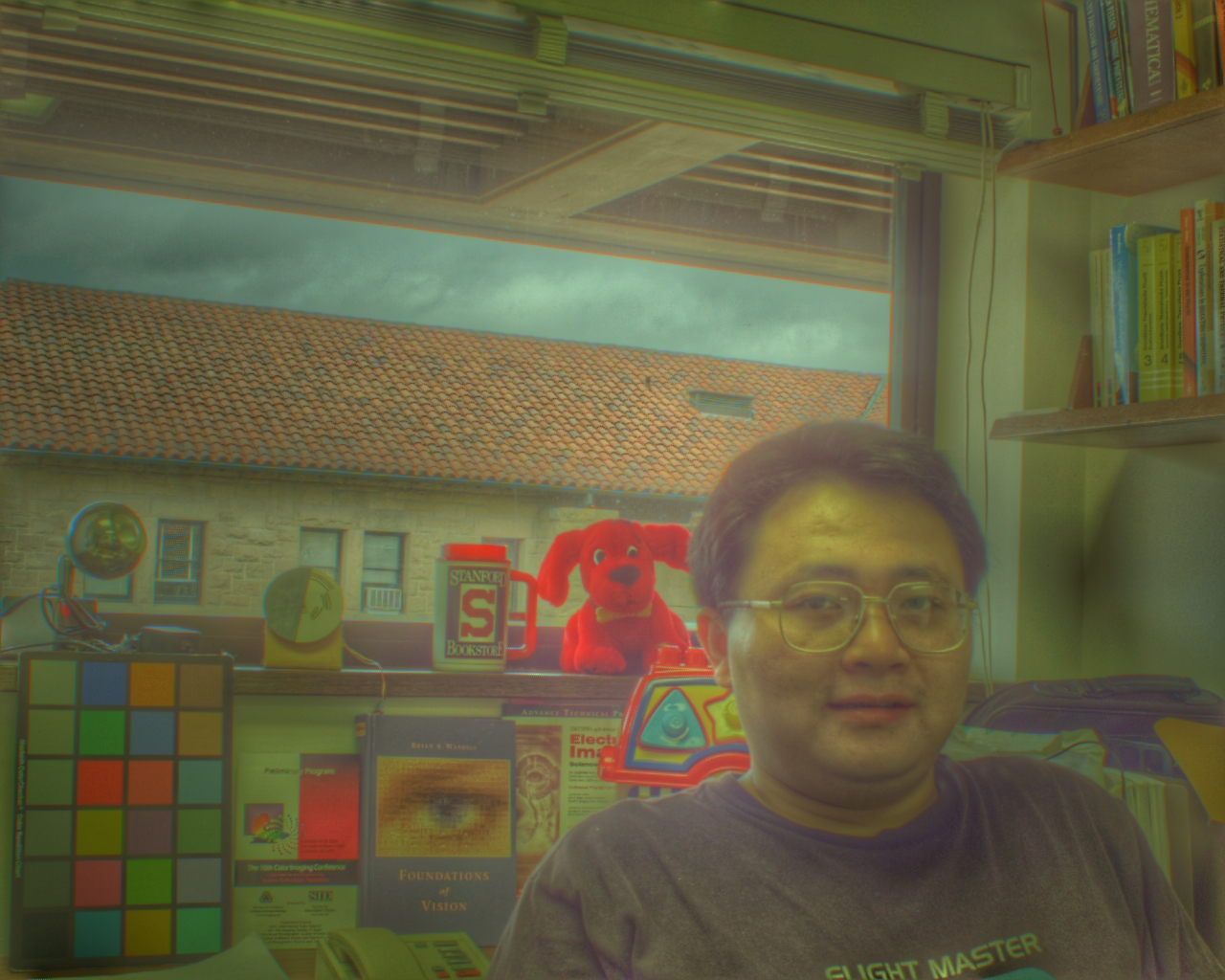 |
The OfficeLightsOffPerson image went from a dynamic range of 3.76 to 0.77 log units, using alpha = 0.2, beta = 0.85, and s = 0.6.
 |
 |
 |
 |