NOTE: The algorithm for gradient-based dynamic range compression is described roughly here.
For more details, see the MATLAB source code in Appendix I, and the original paper by
Fattal, Lischinski, and Werman. (I have included a direct link in the references.)
The algorithm proceeds as follows:
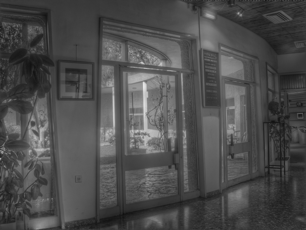
- Take the logarithm of the image intensity, and store it in a matrix, H.
(For color images, take the logarithm of the luminance channel, Y ~ 0.25*R + 0.50*G +
0.25*B.) Most dynamic range compression algorithms operate in the logarithmic
domain; not only is the logarithm of luminance roughly proportional to perceived
brightness, but gradients in the logarithmic domain correspond to ratios in the
luminance domain ( log(A/B) = log(A)-log(B) ).
|
|
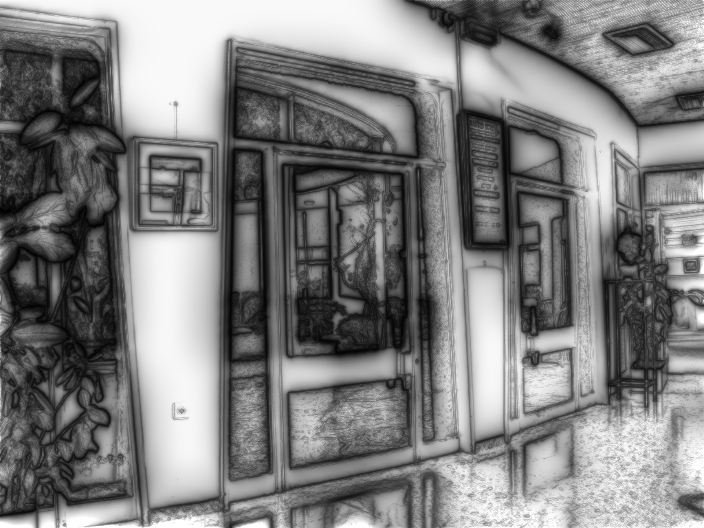
- Compute the gradient attenuation function, PHI.
To compress the dynamic
range of the image while keeping fine details, our attenuation function should be
"progressive" (that is, it should shrink large local gradients more aggressively
than small ones, and it should attenuate gradients that occur over large distances
much more than those that occur only over short distances).
To do this, we form a Gaussian pyramid of H so that we can examine it at
various spatial resolutions. At each level of the pyramid, Hk, we
form an attenuation mapping phik, where each value is a function
of the magnitude of the gradient at that point:
phik(x,y) =
( ||grad(Hk(x,y)|| / (a*2k) )b-1
In the above equation, a and b are user-defined parameters.
a determines the attenuation threshold; all gradients of magnitude less
than a will go roughly unchanged. b is a parameter between 0 and 1
that determines how quickly the attenuation ramps up as gradients get larger.
Fattal et. al recommend an a of roughly 0.1 times the average gradient
magnitude, and a b between 0.8 and 0.9.
Also, note the factor of 2k in the denominator; that is there to
correct for the fact that an average gradient gradavg(H) over
2k pixels in the original image will appear as a gradient
grad(Hk) = 2k*gradavg(H)
over a single pixel in Hk.
Finally, we compose all the different phiks: starting from the smallest
level of the pyramid, we take the corresponding phik, upsample it, then
multiply it componentwise with the next attenuation level up, phik-1.
We continue doing this until we have a final attenuation map, PHI, of the same size
as the original, full-resolution image.
|
|
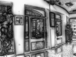
- Compute the desired logarithmic gradient function, G = grad(H)*PHI.
Since all the terms of PHI are positive, the discrete vector field G will point
in the same direction as grad(H) at every pixel, but the largest gradient magnitudes
will be significantly curbed, and we will generally see smaller gradients connecting
global bright and dark regions.
By applying the precomputed attenuation function only at the full-resolution level
(instead of applying the attenuation at each resolution level, then composing the
resulting images), is what saves this algorithm from the halo artifacts that
typically plague multi-resolution TROs.
|
|
- Find the logarithmic image I whose gradient field is closest to G.
At this point, we've determined a reduced vector field, G, which we hope to make the
gradient field of our new, low dynamic range image. Unfortunately, because the
attenuation function we used was nonlinear, G will not generally be a conservative
vector field (in other words, there is no image that could give rise to G as its gradient
field). Fortunately, it is possible to solve for the logarithmic image whose vector
field has the least mean-squared error with G; solving the Poisson equation laplacian(I)
= div(G), results in the appropriate image, I. (See the original paper for a full
explanation.)
There are a couple of ways of going about solving this equation. I opted to use a
rapid Poisson solver with Dirichlet boundary conditions set to zero. This solver is
based on the observation that a 5-point discrete Hessian matrix is block-diagonalizable
by blocks of discrete sine transform coefficients. This allows us to decompose the
problem into M smaller (tridiagonal) problems along each row of the Hessian matrix, each
of which is exponentially easier to compute than the original Hessian matrix inversion.
(For more details, see the references on FFT applications.)
While using a multigrid algorithm might perform somewhat better for large problems (O[N]
complexity versus O[NlogN]), the Poisson solver is still a very efficient algorithm and less
complicated to implement than the multigrid algorithm.
|
|
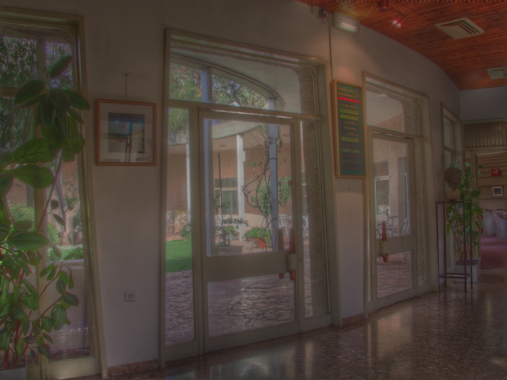
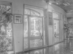
- Exponentiate I to get your final luminance image, Yout.
Recall that we have been working entirely in the logarithmic luminance domain.
To get back the final luminance image for display, simply take the exponential
of each pixel in I. (Note that if you want your values to fall between 0 and 1,
an easy way to do that is to shift the values of I so that they are all negative
before you carry out the exponentiation).
|
|
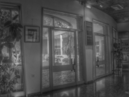
- If your original image was in color, use Yout to reassign color
intensities.
For each color component Ci, define the output color using
Ci,out = (Ci,in/Yin)sYout
where s is a user-defined quantity that determines color saturation. The
original authors recommended values for s between 0.4 and 0.6.
|

|
|