.
So we have now related each discrete component, that is the nth frequency component shifted by k, to the continuous representation shifted by k. This becomes important.
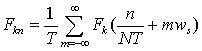
Now we relate the DFT to the CFT with the "aliasing relationship":
.
So we have now related each discrete component, that is the nth frequency
component shifted by k, to the continuous representation shifted by k.
This becomes important.
Now is the part where we make the assumption that F(w) is bandlimited.
We do this by saying that F(w) = 0 for all w such that |w| > L * ![]()
This enables us to write:
.
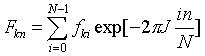
where
.![]() which
we note is a relation bewteen the DFT and the CFT
which
we note is a relation bewteen the DFT and the CFT
.![]() which
comes from the combinations of exponentials
which
comes from the combinations of exponentials
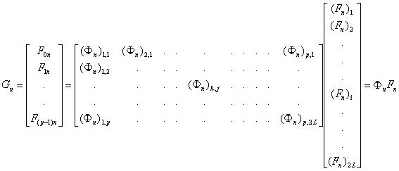
We notice that the matrix ![]() is
something we already know. We can calculate that with a DFT from
the original data. We notice also that
is
something we already know. We can calculate that with a DFT from
the original data. We notice also that ![]() is a matrix that we can calculate simply knowing N, T, L, and all
is a matrix that we can calculate simply knowing N, T, L, and all ![]() .
.
Note that ![]() is a matrix containing 2L points. We have not yet determined
the value of L.
is a matrix containing 2L points. We have not yet determined
the value of L.
Clearly now, what we wish to solve for is ![]() .
We can do this using a number of matrix techniques, which are described
in the paper, but which we will not go into here in the 1D case.
.
We can do this using a number of matrix techniques, which are described
in the paper, but which we will not go into here in the 1D case.
Once we have solved this matrix equation, what do we do now? We
have values for this matrix ![]() ,
but what do these numbers mean? By definition, they are the values
of the continuous Fourier Transform at the point:
,
but what do these numbers mean? By definition, they are the values
of the continuous Fourier Transform at the point:
.![]()
So we have taken these 2L values and assigned w coordinates to them
in the frequency domain as sample point of the frequency representation
of the continuous ideal image. Now again, the matrix equation above
considers only the nth component of all p of our DFTs. We have N-1
more matrix equations to solve, and thus 2L*(N-1) more points to add to
our frequency representation of the continous ideal image. In total,
we will have 2LN points in our representation, whereas we started out with
N (being the most points we could obtain from any one image.) So
we see that our resolution has increased by a factor 2L! If we want
a resolution increase of 2, we make L=1. In general, we will use
small-ish values of L, so perhaps the picture of the matrix equation above
is misleading, but it was purposely drawn that way to illustrate the matrix
multiplication relationships.
Of course, in order to recover the exact image exactly, we would need enough points to be above the Nyquist frequency with respect to the variations of the signal as it reaches the "camera". Nonetheless, we know that the more points we add to the bandlimited frequency representation, the more accurately we will be able to determine the signal in the space domain.
Once we have finished mapping all points from all n into frequency space, we use an inverse Fourier Transform to obtain our higher resolution image.