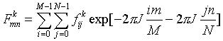
Also note that i
Note, by definition, if k![]() [0,p-1],
then
[0,p-1],
then ![]()
Also note that i![]() [0,
M-1] and j
[0,
M-1] and j![]() [0,N-1]
[0,N-1]
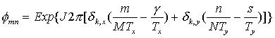
Now we relate the DFT to the CFT with the 2D version of the "aliasing
relationship":
.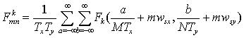
So we have now related each discrete component, that is the (m,n)th
frequency component shifted by k, to the continuous representation shifted
by k. This again becomes important.
Again we make the assumption that F(u,v) is bandlimited in both directions.
We do this by saying that F(u,v) = 0 for all w such that |u| > ![]() *
*![]() and |v|>
and |v|>![]() *
*![]()
This enables us to write another matrix equation:
.![]()
We will not draw the matricies together as we did last time.
We will now however, examine each matrix individually.
.....beginning with
.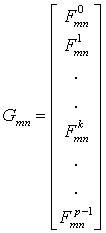
so ![]() which we already know from the DFT. This vector is of length p.
which we already know from the DFT. This vector is of length p.
Now we look at........
.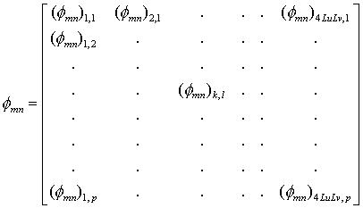
where
.
so we see that this too is something we can readily calculate.
This matrix is of size p x 4![]()
![]()
In this paper, methods are desribed to circumvent the direct calculation
of both of the above matricies. As we will now see, we desire to
find the values of ![]() ,
which can be obtained more readily by noting some symmetries of the above
matricies.
,
which can be obtained more readily by noting some symmetries of the above
matricies.
Now we look at.......
.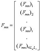
where
.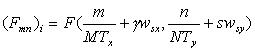 which
we note is a relation bewteen the CFT at a given point in
which
we note is a relation bewteen the CFT at a given point in
continuous space and values from the DFT. This vector is
4![]()
![]() in length
in length
.![]()
.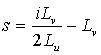
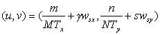
and we now see that we can calculate exatly the continuous (u,v) coordinate
at which to put the value ![]()
Note that ![]() is a matrix containing 4
is a matrix containing 4![]()
![]() points. We have not yet determined the values of
points. We have not yet determined the values of ![]() and
and ![]() .
.
Once we have solved this matrix equation, what do we do now? We
have values for this matrix ![]() ,
but what do these numbers mean? As with in the 1D case, these are
values of the continuous Fourier Transform at a given (u,v) point
,
but what do these numbers mean? As with in the 1D case, these are
values of the continuous Fourier Transform at a given (u,v) point
.
So we have taken these 4![]()
![]() values and assigned (u,v) coordinates to them in the frequency domain as
sample point of the frequency representation of the continuous ideal image.
Now again, the matrix equation above considers only the (m,n)nth component
of all p of our DFTs. We have (N-1)(M-1) more matrix equations to
solve, and thus 4
values and assigned (u,v) coordinates to them in the frequency domain as
sample point of the frequency representation of the continuous ideal image.
Now again, the matrix equation above considers only the (m,n)nth component
of all p of our DFTs. We have (N-1)(M-1) more matrix equations to
solve, and thus 4![]()
![]() (N-1)(M-1)
more points to add to our frequency representation of the continous ideal
image. In total, we will have 4
(N-1)(M-1)
more points to add to our frequency representation of the continous ideal
image. In total, we will have 4![]()
![]() MN
points in our representation, whereas we started out with MN (being the
most points we could obtain from any one image.) So we see that our
resolution has increased by a factor 4
MN
points in our representation, whereas we started out with MN (being the
most points we could obtain from any one image.) So we see that our
resolution has increased by a factor 4![]()
![]() !
If we want a resolution increase of 2 in each direction (and thus 4 overall),
we make
!
If we want a resolution increase of 2 in each direction (and thus 4 overall),
we make ![]() =
=![]() =1.
In general, we will use small-ish values of L.
=1.
In general, we will use small-ish values of L.
Of course, in order to recover the exact image exactly, we would need enough points to be above the Nyquist frequency with respect to the variations of the signal as it reaches the "camera". Nonetheless, we know that the more points we add to the bandlimited frequency representation, the more accurately we will be able to determine the signal in the space domain.
Once we have finished mapping all points from all n into frequency space,
we use an 2D inverse Fourier Transform to obtain our higher resolution
image.