Zernike
Polynomials and Their Use in Describing the Wavefront Aberrations of the Human
Eye
Psych 221/EE 362 Applied Vision and Imaging Systems
Course Project, Winter
2003
Patrick Y. Maeda
Stanford University
Introduction
Currently there is considerable interest in correcting the higher-order optical aberrations of the human eye [1]. Present-day laser eye surgery techniques like PRK and LASIK correct only defocus and astigmatism, which are 2nd order aberrations. Surgically correcting the additional higher-order aberrations could extend the limits of human vision beyond 20/20. In addition, this type of capability could be used to eliminate the higher-order aberrations that may have been caused by a prior surgical procedure. These induced aberrations are responsible for the glare, halos, and other visual defects that have been reported by some eye surgery patients.
Another application involves the high-resolution imaging of the retina and other structures (rods, cones, nerve fibers, blood vessels, capillaries, pigment cells, etc.,) using adaptive optics for the diagnosis and treatment of eye disorders [1].
To determine and apply the proper correction that will eliminate or minimize these aberrations, their characteristics must first be captured and quantitatively described. The wave aberration function suits this purpose well because it completely describes the aggregate effects of the cornea and lens on light passing through every location in the pupil. It defines how the phase of the light is affected after it has propagated through the optical system. In the case of laser eye surgery, if you know the wave aberration function, you know what must be done to the refractive properties of the eye to create an image on the retina that is limited only by diffraction and scattering. For retinal imaging with adaptive optics, if you know the wave aberration function, you know what must be done to the light entering the pupil to create an image on the retina that is limited only by diffraction and scattering [2].
Understanding what is needed to correct defocus and astigmatism can be accomplished by having patients view targets through sets of sphero-cylinder test lenses. However, determining the other higher order wave aberrations requires more sophisticated techniques. Wavefront measuring instruments like the Shack-Hartmann Sensor are being utilized to provide data from which the wave aberrations of the human eye can be accurately and reliably estimated.
For the above reasons a mathematical formulation is needed, not only to quantitatively describe the aberrations, but also to facilitate accurate estimation of the wave aberration function from measurement data. In response to the perceived need in the vision community, the Optical Society of America formed a task force and charged it with the mission of developing recommendations on definitions, conventions, and standards for the reporting of optical aberrations of human eyes. One major outcome has been a recommendation adopting the use of Zernike Polynomials for this purpose [3].
The objectives of this course project include an explanation of why Zernike polynomials are preferred over other functions, a mathematical definition of Zernike polynomials, their use in describing the wave aberration function, a simulation showing the effects of the higher order aberrations on image quality, and an illustration of how Zernike polynomials are used to estimate the wave aberration function from measurement data.
General Optical System Description
|
Figure 1. Coordinate System |
Figure 2. Optical System Components |
The physical layout for imaging consists of an object plane, an optical system, and an image plane as shown in Figure 1. Right-handed coordinate systems are commonly employed. A typical optical system, illustrated in Figure 2 consists of lenses and an aperture. The aperture limits the amount of light passing through the optical system. The pupils of the optical system are the images of the physical aperture as formed by the front and rear sections of the optics. The Entrance Pupil is the image of the aperture formed by the optics in front of the aperture, while the Exit Pupil is the image of the aperture formed by the optics in back of the aperture. For the particular system shown in Figures 3 and 4, these pupils are virtual images of the aperture. The Exit and Entrance pupil size and location are independent of object and image locations in many systems. Notable exceptions are wide-angle lenses and fisheye lenses.
|
Figure 3. Pupils of an Optical System |
Figure 4 shows the geometrical ray trace for a distant point object. The geometrical rays are normal to the wavefronts. Wavefronts are surfaces of constant phase. As seen in the figure, light from the object initially heads toward the Entrance Pupil, while the light exiting the optical system appears to emanate from the Exit Pupil. This ray trace is for a system with no aberrations, so after propagating through the entire system, the wavefronts are perfectly spherical and the rays converge to a point. Real optical systems, however, are not aberration free and the wavefronts, which are surfaces of constant phase, deviate from sphericity. This illustrates the fact that aberrations introduce phase distortions into the light waves. In addition, the effects of diffraction must also be taken into account.
Note that the light forming the image completely fills the Exit Pupil. Also, since the Exit Pupil is the aperture as seen from the image space of the optical system, all of the effects of aberrations in the system are fully contained in the light distribution at the Exit Pupil. The Exit Pupil therefore is good place to define and characterize the nature of the light in an image forming optical system. Once we know the distribution of light (i.e., amplitude and phase) at the Exit Pupil, we can calculate the impulse response or point spread function (PSF) of the optical system using the diffraction integral and Fourier optics techniques [4, 5]. This fully accounts for the effects of both aberrations and diffraction.
Monochromatic Wavefront Aberrations
Snell’s law governs the refraction of light at optical surfaces. It involves the use of the sine function, which is non-linear.
|
|
(1) |
In paraxial systems, angles are small, sin(φ) ~ φ, and we have first-order optics, no aberrations, and spherical wavefronts. In non-paraxial systems, higher order terms in the power series expansion of the sine function can be significant, and aberrations are no longer negligible. The non-zero aberrations cause wavefronts to deviate from sphericity. Non-zero aberrations occur even when refracting surfaces of lenses are perfectly spherical. Non-zero aberrations occur even for a perfect plane-parallel plate in a converging or diverging beam of light because Snell’s law is non-linear.
We therefore expect the wave aberration function to be expressible as power series expansions or polynomials. For example, a weighted sum of basis functions, monomials, or modes, which are functions of the pupil coordinates.
The wave aberration function, W(x,y), is defined as the distance, in optical path length (product of the refractive index and path length), from the reference sphere to the wavefront in the exit pupil measured along the ray as a function of the transverse coordinates (x,y) of the ray intersection with a reference sphere centered on the ideal image point. It is not the wavefront itself but it is the departure of the wavefront from the reference spherical wavefront as indicated in Figure 5.
|
Figure 5. Wave Aberration Function for a distant point object |
A standard way of describing the wave aberration is to use a Taylor expansion polynomial in field (object height) and pupil coordinates [6].
|
|
(2) |
Some conventions suppress the image height by absorbing it into the wave aberration coefficients. The wave aberration polynomial is also typically expressed in terms of the normalized pupil radius, ρ :
![]()
However, the terms in the Taylor series do not form an orthogonal set of basis functions and therefore are not recommended for data fitting and describing experimental measurements of wavefront aberrations [7].
Optical materials exhibit dispersion, the variation of refractive index with wavelength. So in addition to the monochromatic aberrations there are chromatic aberrations, where each wavelength or spectral band has its own wave aberration function. The final image, therefore, is a superposition of the spectral images over the entire waveband each affected by the set of monochromatic aberrations occurring at each wavelength.
The Effects of Aberrations on Image Quality
Aberrations negatively impact image quality. They change the size and shape of impulse response or point spread function (PSF), which blurs the image. In terms of frequency analysis, the frequency response of the optical system is reduced by phase distortion within the passband.
The effects of aberrations can therefore be characterized by calculating the PSF or MTF (Modulation Transfer Function) of the optical system.
Calculating the PSF and MTF
The image of a point object formed by the optical system is the point spread function or impulse response. It is defined as [4, 5]:
|
|
(3) |
The Modulation Transfer Function is modulus of the Optical Transfer Function. The OTF and MTF are given by [4, 5]:
|
|
(4) (5) |
The OTF can also be calculated as the auto-correlation of the generalized pupil function, but because the FFT will be used for computational efficiency, the OTF will be calculated using the Fourier transform of the PSF.
For visual applications it is often more convenient to express the PSF and MTF in terms of visual angle. These expressions are given by [8]:
|
|
(6) (7) |
|
|
(8) (9) |
The calculations and computational domains are illustrated in Figures 6 and 7.
|
Figure 6. PSF Calculation and Computational Domains |
|
Figure 7. MTF Calculation and Computational Domains |
Why Use Zernike Polynomials?
Optical system aberrations have historically been described, characterized, and catalogued by power series expansions, where the wave aberration is expressed as a weighted sum of power series terms that are functions of the pupil coordinates. Each term is associated with a particular aberration or mode. For example, spherical aberration, coma, astigmatism, field curvature, distortion, and other higher order modes.
Many optical systems have circular pupils. So many analyses and calculations (e.g. diffraction) will involve the integration of the pupil function and wave aberration function over a circular pupil. Experimental measurements will also be performed over a circular pupil and will commonly require some form of data fitting. It is, therefore, convenient to expand the wave aberration in terms of a complete set of basis functions that are orthogonal over the interior of a circle. Experimental data can be fit to a weighted sum of these orthogonal basis functions.
Zernike polynomials form a complete set of functions or modes that are orthogonal over a circle of unit radius and are convenient for serving as a set of basis functions. This makes them suitable for accurately describing wave aberrations as well as for data fitting. They are usually expressed in polar coordinates, and are readily convertible to Cartesian coordinates. These polynomials are mutually orthogonal, and are therefore mathematically independent, making the variance of the sum of modes equal to the sum of the variances of each individual mode. They can be scaled so that non-zero order modes have zero mean and unit variance. This puts all modes in a common reference frame that enables meaningful relative comparison between them.
Different Zernike polynomial definitions are currently in use. The convention adopted by the OSA has x “horizontal”, y “vertical”, and θ is measured counter-clockwise from x-axis (i.e. right-handed coordinate system). More traditional notation measures θ clockwise from y-axis.
There is the Orthogonal type where the polynomials are normalized to have unity magnitude at edge of pupil. There is also the Orthonormal type where the terms are normalized so that the coefficient of a particular term or mode is the RMS contribution of that term. The Orthonormal set of Zernike polynomials is recommended for describing wave aberration functions and for data fitting of experimental measurements for the eye [3]. The Orthonormal set is adopted as the Standard definition of Zernike polynomials in this project.
Standard Set of Zernike Polynomials
Zernike polynomials are normally expressed in polar coordinates (ρ ,θ ) where 0 < ρ < 1, 0 < θ < 2π . Figure 8 shows the coordinate system of the unit circle over which they are defined. Conversion to rectangular coordinates may be desirable for some applications.
|
Figure 8. Pupil Coordinate Systems |
Each polynomial has three components: the normalization factor, a radially dependent polynomial, and an azimuthally dependent sinusoid. A double indexing scheme is used where: n is the highest power or order of the radial polynomial and m is the azimuthal or angular frequency of the sinusoidal component. An accompanying single indexing scheme is also employed where the index j is used to indicate mode number.
The Zernike polynomials are defined as [3]:
|
|
(10) (11) (12) |
Table 1 contains a list of Zernike polynomials up to order 4 and their meanings relative to the traditional Seidel or Primary aberrations [3, 9, 10].
|
Table 1. Zernike Polynomials (up to 4th order) |
Comparison with the terms in equation (2) shows that the functional form of the traditional wave aberration terms or modes are represented in the various Zernike polynomials.
There
are occasions when expressing the Zernike polynomials in rectangular form is
needed. For example, data from the
Shack-Hartmann Wavefront Sensor represent the partial derivatives of the wave
aberration as a function of x and y.
The formulas for conversion to rectangular coordinates and the various
indices are provided below:
|
|
|

Describing the Wave Aberration Function using Zernike Polynomials
The wave aberration function is expressed as a weighted sum of Zernike polynomials [7]:
|
|
(13) |

Results and Discussion
Two Matlab functions, factorial.m and zernike.m were written to implement equations (10) – (12) and generate values for any Zernike polynomial specified by n, m, x, y, and d. Where x and y are 1-D arrays of the x-coordinate and y-coordinate pupil values, and d is the pupil diameter. A Matlab script, ZernikePolynomial.m, was created to generate an image and surface plot of any Zernike polynomial specified by n, m, x, y, and d. Figure 9 contains the images of Zernike polynomials, generated by ZernikePolynomial.m, up to 6th order in a pyramid arrangement.
Two Matlab scripts, ZernikePolynomialPSF.m and ZernikePolynomialMTF.m utilize equations (6) – (9) to generate and plot the PSF and MTF for any wave aberration mode associated with any Zernike polynomial specified by n, m, pupil diameter (3 to 8 mm), RMS wavefront error (in microns), and wavelength (in nm). These scripts were used to generate the corresponding PSF and MTF images and plots for the wave aberration modes up to 6th order corresponding to each of the Zernike polynomials in Figure 9.
Figure 10 shows the PSF images for a 4 mm pupil diameter at λ = 570 nm and an RMS wavefront error equal to 0.3 micron = 0.53 λ. The PSFs were scaled to achieve saturation to make the fine spatial structure more visible in the images.
Figures 11 and 12 plot the MTFs, up to 6th order for 4 mm and 7.3 mm pupil diameters at λ = 570 nm, and an RMS wavefront error equal to 0.114 micron = 0.2 λ . An RMS wavefront error of 0.07 λ or lower is considered diffraction limited, i.e. the aberration is small enough so effectively the light is only affected by diffraction.
|
|
|
Figure 9. Zernike Polynomials up to 6th Order |
|
|
|
Figure 10. PSFs of Wave Aberrations Corresponding to Each Zernike Mode up to 6th Order, 4 mm Pupil Diameter, RMS Wavefront Error = 0.53 λ (Images are saturated to bring out fine structure in PSFs) |
|
|
|
Figure 11. MTFs of of Wave Aberrations Corresponding to Each Zernike Mode up to 6th Order, 4 mm Pupil Diameter, RMS Wavefront Error = 0.2 λ |
|
|
|
Figure 12. MTFs of of Wave Aberrations Corresponding to Each Zernike Mode up to 6th Order, 7.3 mm Pupil Diameter, RMS Wavefront Error = 0.2 λ |
The simulation images and plots show how the various Zernike modes affect the PSF and MTF relative to an unaberrated system. In all cases, with the exception of the piston modes, the image quality will be degraded. The piston mode (n = 0, m = 0) simply produces a uniform phase shift across the pupil and therefore the PSF and MTF are the same as that of an unaberrated system. The tilt modes (n = 1, m = -1, 1) are linear phase gradients across the pupil and result in an x or y shift in the PSF, but do not affect the size or shape of the PSF and therefore the MTF is not affected. Note also for a given RMS wavefront error level, the MTF usually gets worse as the mode order gets higher.
These particular plots show that the MTFs for the 7.3 mm pupil are better than those for the 5.4 mm pupil. This is because the RMS wavefront error is the same for both pupil sizes but the diffraction effects are worse for the smaller pupil. In a real optical system, the wavefront errors typically increase with pupil size significantly beyond the diffraction limit and so the MTF worsens with increased pupil diameter.
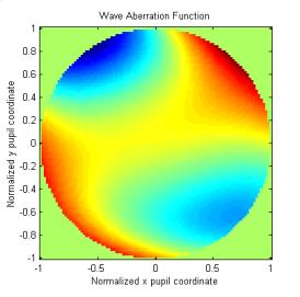
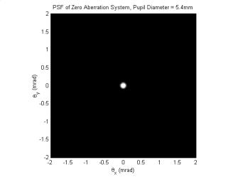
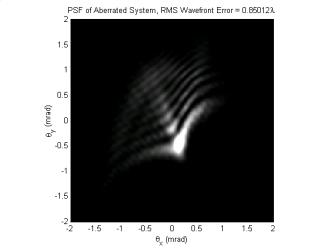
Matlab scripts, WaveAberration.m, WaveAberrationPSF.m, and WaveAberrationMTF.m utilize equation (13) to generate the wave aberration function. These scripts compute and plot W(ρ ,θ ) the PSF, and the MTF for a wave aberration function made up of a weighted sum of Zernike polynomials. Each polynomial is weighted by an RMS wave aberration coefficient. These coefficients are determined from the Wavefront sensor measurements. Table 2 lists the wave aberration coefficients determined from a Wavefront sensor measurement of a patient with a pupil diameter of 5.4 mm [11]. The System or Total RMS wavefront error is the square root of the sum of the squares of the individual RMS coefficients. In this particular case only the Zernike polynomials up to and including the 4th order terms were used to fit the data from the wavefront sensor. Figure 13 plots the wave aberration function. Figure Figures 14 to 15 show the results of the PSF and MTF simulations of the patient data.
From a review of the coefficients in Table 2, we see that errors attributable to defocus and tilt are zero, and the ± 45º astigmatism mode (j = 3, n = 2, m = -2) dominates. A quick comparison shows that the wave aberration image in Figure 13 is similar to the image of the n = 2, m = -2, Zernike polynomial in Figure 9 as expected. The total RMS wavefront error is 0.85 λ , which is more than 10 times the diffraction limit (~ 0.05 λ to 0.07 λ). The MTF plots in Figure 15 indeed show that the optical system has been significantly degraded below diffraction limit performance levels.
|
|
|
|
Table 2. Measured Wave Aberration Coefficients [11] |
Figure 13. Wave Aberration Function |
|
|
|
|
Figure 14. PSF of Eye with Zero Aberrations |
Figure 15. PSF of Aberrated Eye |
|
|
|
Figure 15. MTF of Aberrated Eye |
Wavefront Aberration Measurement
So how is the wavefront aberration function of the eye actually measured? One issue is that there is no physical access to the retinal plane or the exit pupil of the eye in a manner similar to what is shown in Figures 4 and 5. To get around this problem, the system is turned around, as shown in Figure 15, and the principle of reversibility is invoked. A small focused spot of light is formed on the retina of the eye and the reflected light serves as a point source. The reflected light propagates back through the optics of the eye and a wavefront sensor can measure the exiting light.
|
|
|
Figure 15. Basic Set-up for Measuring the Aberrations of the Eye |

The wavefront aberration function determined from this measurement can be used to determine the corrections that need to be made to the eye. Reversibility tells us that if the optics of the eye is corrected so that an exiting planar wavefront is formed (within the limits of diffraction) from a point source on the retina, then a planar wavefront entering the eye will form a spot on the retina that is limited only by the effects of diffraction.
The problems associated with the double-pass nature of the light propagation are mitigated by a couple of factors. The incoming beam diameter can be made small enough so that the aberrations from the first pass through the optics will be minimal. The spot size diameter on the retina from a 3 mm diameter beam will be on the order of 5 microns. If the diffusely reflected light is used for the wavefront measurement, the phase error associated with the first pass is lost and is not contained in the reflected light, as it would be with a specular reflection at the retina [10]. If the light beam entering the eye is polarized, using a polarization beam splitter can separate the diffuse and specularly reflected light. Diffuse reflections are unpolarized, while the specular reflections remain polarized.
A schematic layout of the Shack-Hartmann Wavefront Sensor is shown in Figure 16. A polarized light source is used to produce a small spot on the retina. The diffuse reflected light that propagates back through the lens and cornea and out of the eye is relayed to the plane of the lenslet array. Any specularly reflected light will be reflected out of the return path by the polarization beam splitter (PBS). The relay optics is used to image the pupil of the eye onto the plane of the lenslet array.
|
|
|
Figure 16. Shack-Hartmann Wavefront Sensor Schematic Layout |
|
|
|
Figure 17. Shack-Hartmann Sensor Lenslet Array |
The wavefront at the lenslet array will be aberrated as shown in Figure 17. The lenslet array will convert the local sections of the wavefront into focused spots at the CCD. If the incident wavefront is a perfect plane then the focused spots will not be displaced from the optical axes of the various lenslets. An aberrated incident wavefront will produce a non-zero spot displacement. So for each lenslet there will be an x-displacement, Δx, and a y-displacement, Δy. The displacements divided by the focal length of the lenslet is equal to the local slope of the wavefront. The displacement data measured by the CCD can now be fit to a Zernike polynomial expansion where the expansion coefficients are determined using Least-squares estimation as outlined below [10].
|
|
|
|
|
|
Conclusion
In conclusion, I learned that Zernike Polynomials are well suited not only for describing the wave aberration functions of optical systems with circular pupils, but also for estimating the wave aberration coefficients from wavefront measurements. The project provided me with the opportunity to apply what I have learned about the optical system of the human eye in this course along with the optical systems and Fourier optics material from previous courses. Linear systems theory made the mathematics and computation of image formation and image quality evaluation relatively straightforward.
Suggestions for future work include extending the simulation to incorporate chromatic effects, investigating the changes in the wave aberration of the eye with accommodation, running more simulations on a wide set of patient data, simulating the higher order aberrations induced by the PRK and LASIK procedures, and researching some of the new wavefront technologies like implantable lenses.
Appendix I
Matlab Source Code:
Other:
Project Summary Powerpoint Presentation
References
[1] MacRae, S. M., Krueger, R. R., Applegate, A. A., (2001), Customized Corneal Ablation, The Quest for SuperVision, Slack Incorporated.
[2] Williams, D., Yoon, G. Y., Porter, J., Guirao, A., Hofer, H., Cox, I., (2000), “Visual Benefits of Correcting Higher Order Aberrations of the Eye,” Journal of Refractive Surgery, Vol. 16, September/October 2000, S554-S559.
[3] Thibos, L., Applegate, R.A., Schweigerling, J.T., Webb, R., VSIA Standards Taskforce Members (2000), "Standards for Reporting the Optical Aberrations of Eyes," OSA Trends in Optics and Photonics Vol. 35, Vision Science and its Applications, Lakshminarayanan,V. (ed) (Optical Society of America, Washington, DC), pp: 232-244.
[4] Goodman, J. W. (1968). Introduction to Fourier Optics. San Francisco: McGraw Hill
[5] Gaskill, J. D. (1978). Linear Systems, Fourier Transforms, Optics. New York: Wiley
[6] Fischer, R. E. (2000). Optical System Design. New York: McGraw Hill
[7] Thibos, L. N.(1999), Handbook of Visual Optics, Draft Chapter on Standards for Reporting Aberrations of the Eye. http://research.opt.indiana.edu/Library/HVO/Handbook.html
[8] Bracewell, R. N. (1986). The Fourier Transform and Its Applications. McGraw Hill
[9] Mahajan, V. N. (1998). Optical Imaging and Aberrations, Part I Ray Geometrical Optics, SPIE Press
[10] Liang, L., Grimm, B., Goelz, S., Bille, J., (1994), “Objective Measurement of Wave Aberrations of the Human Eye with the use of a Hartmann-Shack Wave-front Sensor,” J. Opt. Soc. Am. A, Vol. 11, No. 7, 1949-1957.
[11] Liang, L., Williams, D. R., (1997), “Aberration and Retinal Image Quality of the Normal Human Eye,” J. Opt. Soc. Am. A, Vol. 14, No. 11, 2873-2883.