Resolution in Color Filter Array Images

Jon Peterson and Cobus Heukelman

[Introduction] [Background and Prior Work] [Methodology] [Results] [Conclusion] [References] [Appendix]

Downloadable Content

Introduction

Ever since the digital camera was first invented, there has been a drive to pack more and more pixels into a single sensor. The most common color filter array (CFA) used is the Bayer mosaic, which consists of one red, two green and one blue filter in a square 2x2 arrangement. The reason for choosing two green filters is that the eye is most sensitive to changes in green. With the many megapixels available today, there is the possibility of trading off spatial resolution to achieve better performance in other areas such as color reproduction and low light performance. For instance, choosing a color filter array that has more than 3 colors might yield better color reproduction, but at the cost of a lower resolution. In this project we investigate the performance tradeoffs involved when adding more colors to the CFA, and look at what guidelines we can use when selecting colors for a filter array.

Background and Prior Work

Color Architecture

There are many different color architectures that can be used to capture images in digital cameras. In a study by Peter Catrysse et al[1], the following three architectures are compared: (1) using a sensor array that contains an interleaved mosaic of color filters, (2) using dichroic prisms to split the image into different spatially separated copies that are captured and (3) using a time-varying color filter to capture the images sequentially. Of these architectures (1) is the most cost effective and therefore the most widely used. The second architecture requires multiple sensors to record the spatially separated copies, making it much more expensive and the last method requires longer exposure times, since the images are captured one after the other. The CFA architecture is the most prevalent, but this approach was developed at a time when every single pixel was a precious resource for achieving the needed special resolution. Today, digital SLR cameras can have 18 Megapixels or more. Most users do not need this amount of spatial resolution, which raises the question whether it is possible to get an improvement in color reproduction or low light performance by using extra colors in the filter array.

Simulation Tools

The numerous variables in the camera imaging pipeline make it difficult to analyze the different components in practice. This project uses ISET (Image Systems Evaluation Tools)[2] to simulate the entire image processing pipeline. By keeping the rest of the imaging pipeline fixed and adjusting only the sensor, we can evaluate the effect of different sensor designs on the final image.

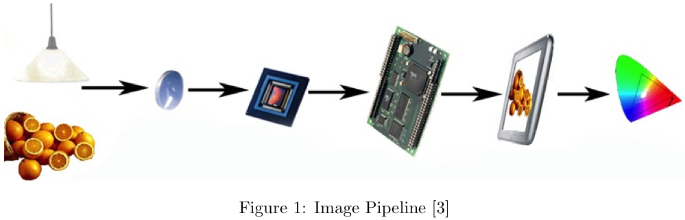
As illustrated in the above image, the simulation software starts with a radiometric description of the scene, containing the spectral radiance at each pixel in the sampled scene. Illumination is applied to the scene and it is then transformed by the optics. This gives a description of the scene at the camera sensor. After sampling by the sensor, the image processor performs demosaicking and color conversion to get the captured scene ready for display.

Color Filter Arrays

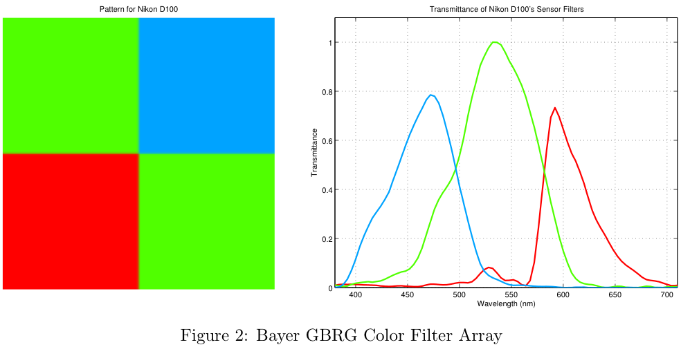
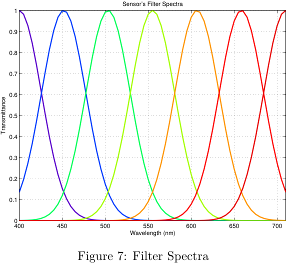
The most common arrangement for a color filter array, called the Bayer pattern is shown below. As can be seen in Figure 2, the pixels of the sensor are covered by red, green and blue filters. The transmittance functions for the filters of a Nikon D100 camera are shown on the right (From ISET).

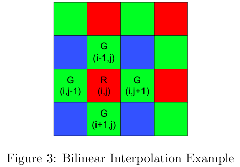
Due to the trichromaticity of color vision we need a red, green and blue value for each pixel, but in the filter array each pixel can only be red, green or blue separately. This means that we need to estimate the missing values, which is known as demosaicking. As described by Joyce Farrell in [2], this is quite a complex problem and there are various methods that have been developed for it. These include methods that interpolate the color planes separately as well as methods that use data from all the color planes in calculating each value. The focus of this project is not directly on these algorithms, but it is nonetheless valuable to know a little about the demosaicking scheme used since it has a large influence on the results. The ISET software used for this project implements a simple bilinear interpolation scheme for demosaicking. This method, as well as a newer high-quality linear method for demosaicking is described by Malvar in [4]. The bilinear method calculates the missing color at a pixel by taking an average of the neighboring pixels that have that color. For instance, the green value of the red pixel "R" in Figure 3 is calculated by taking the average of the surrounding green pixels:

The advantage of this method is that it is very fast to compute, but because it is essentially a convolution operation the resulting image is blurred in all directions. A more advanced way is described by Jim Adams et al in [5]. This adaptive strategy performs edge detection on the neighboring pixels and then averages only along the edges and not across them. By using this bilateral filtering technique the colors are interpolated without blurring the edges.

Methodology

This project consists of two parts. Firstly the problem of defining the filter colors was investigated. This was done both by brute force simulations and then a design rule was used to define the filter spectra. Secondly the problem of defining the spatial pattern for the different color filters within the CFA was investigated.

Color Reproduction

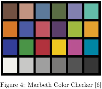
The ability of the color filter array to reproduce the image that is incident on the sensor is evaluated by using a perceptual color metric, namely the CIELAB(1976) delta E value which calculates the perceptual difference between the two images. A perceptual method is used because the only differences that are important to the user are those that can be seen with the human eye. Unfortunately there is no ideal metric that can tell us exactly how the human visual system will see a scene, but for large uniform patches of color, such as the Macbeth chart (Figure 4), the CIELAB metric gives good results. The color reproduction of the CFA is evaluated by using a Macbeth color chart under a known illuminant as the scene, computing the image after processing and comparing the resulting colors to the known values for the Macbeth color chart under that specific illuminant.

Spatial Resolution

In addition to accurately being able to reproduce the color of a scene, it is also important to be able to reproduce any edges in the scene. Edges are particularly important, because we associate "sharp" images as images containing distinctive edges. If the sensor is unable to reproduce strong edges, the resulting image will look blurry. The human visual system is particularly sensitive to the presence or absence of strong edges, since whole areas of the brain are dedicated to edge detection[7].

Figure 5 shows the ISO 12233 Resolution chart[8]. For our analysis, we did not use the entire test chart, instead we focused only on a small area of the chart. The area we focused on was a particular tilted square, we refer to this section as the "slanted bar"[9].

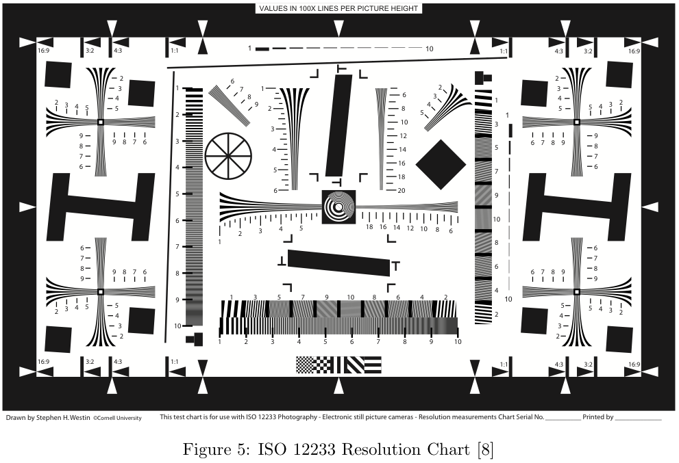
The slanted-bar scene is simply a diagonal line separating a white region and a black region. This scene is a step function which contains very high frequency information. By analyzing the sensor's response to the step function, the sensor's Modulation Transfer Function (MTF) can be generated. The result of generating this MTF is a metric called MTF-50, which is simply the point where the amplitude of the frequency response reaches 50% of the maximum. For our tests,Êwe focus on the MTF-50 metric in order to make comparisons between sensors.

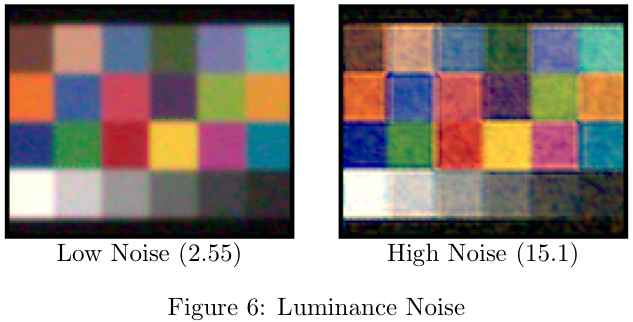
Luminance Noise

The luminance noise is calculated for each of the squares in the grey series of the Macbeth Color Checker. Below is an example of what luminance noise looks like. For high noise there are darker and lighter patches within each square of the color chart.

The luminance noise is calculated as a percentage of the standard deviation of the luminance over the mean luminance in the block.

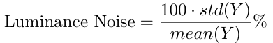
This gives an indication of how uniform the luminance is within a single block.

Defining Filter Colors - Brute Force Simulation

The first approach to defining the filter spectra uses a brute force method to test the performance of many different sensor configurations. By running many simulations the general performance of a sensor with a certain number of filters was determined. For these simulations, the number of filters was varied from 3 to 7. The shape of each filter was defined to be Gaussian, with amplitude 1. By changing the width and the center position of each filter, it is possible to generate many different sensors.

The figure below shows the process for each simulation.

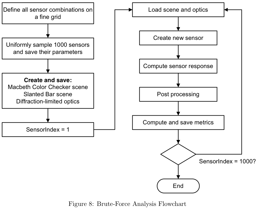
Firstly all the sensor combinations are defined on a fine grid. Next, 1000 of these sensors are uniformly sampled and their parameters are saved. The reason for first using a fine grid to generate many combinations and then sampling this is so that a wider variety of center positions and widths are used in the simulation, giving better statistics. The program then creates and saves the structures for the scene and optics. The reason for this is twofold: Firstly, simulating the optics takes the longest of all the steps in the image pipeline, and by saving this it only has to be computed once. Secondly, by using exactly the same scene and optics for each sensor the variation introduced by the Poisson noise process used to simulate the photons is eliminated.

For each of the 1000 different configurations, a new sensor object is then computed and put through the rest of the image pipeline. After post processing, which includes demosaicking and white balancing, the metrics for the sensor are computed and saved. The metrics that we decided to use to quantify the data are the delta-E values for color accuracy, the MTF-50 for spatial resolution and the luminance noise.

Theory-Based Simulations

In addition to trying a large number of possible filter combinations algorithmically, we tried to come up with a theoretical approach which more closely modeled the response of the human eye. The human eye is not equally sensitive across the entire visible spectrum. Figure 9b shows the individual cone responses as well as the sum of the responses.

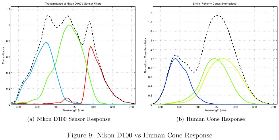
The overall sensitivity of human cones is more sensitive in the middle wavelengths (~550nm) and less sensitive at the extremes (380nm and 710nm). Also notice the overall response of the Nikon D100 (Figure 9a) is much more sensitive in the middle wavelengths and tapers off at the extremes.

For our theoretical approach, we created a set of design rules based on the assumption that the overall sensitivity of the human eye is Gaussian. It is obvious that the overall result is not exactly Gaussian, but it served as an interesting point of discussion.

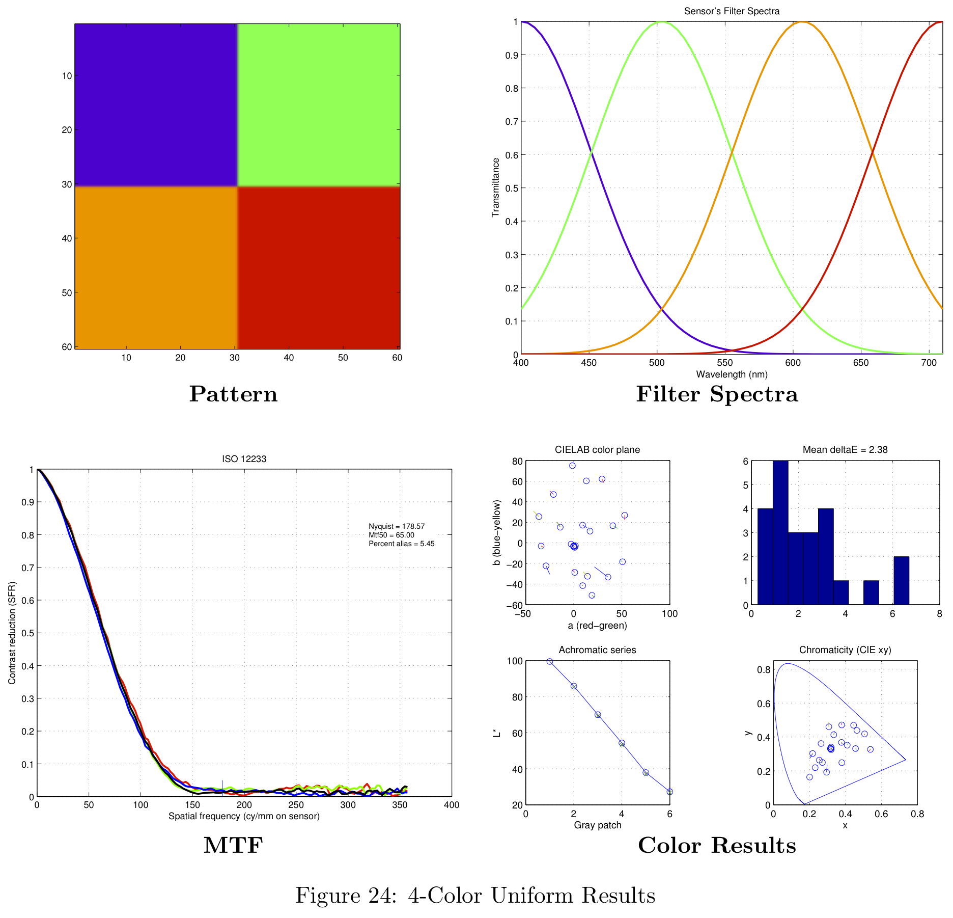
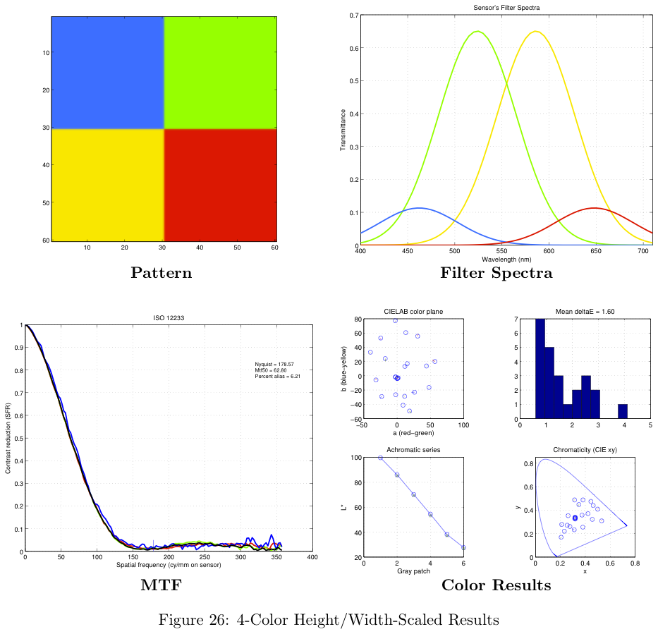
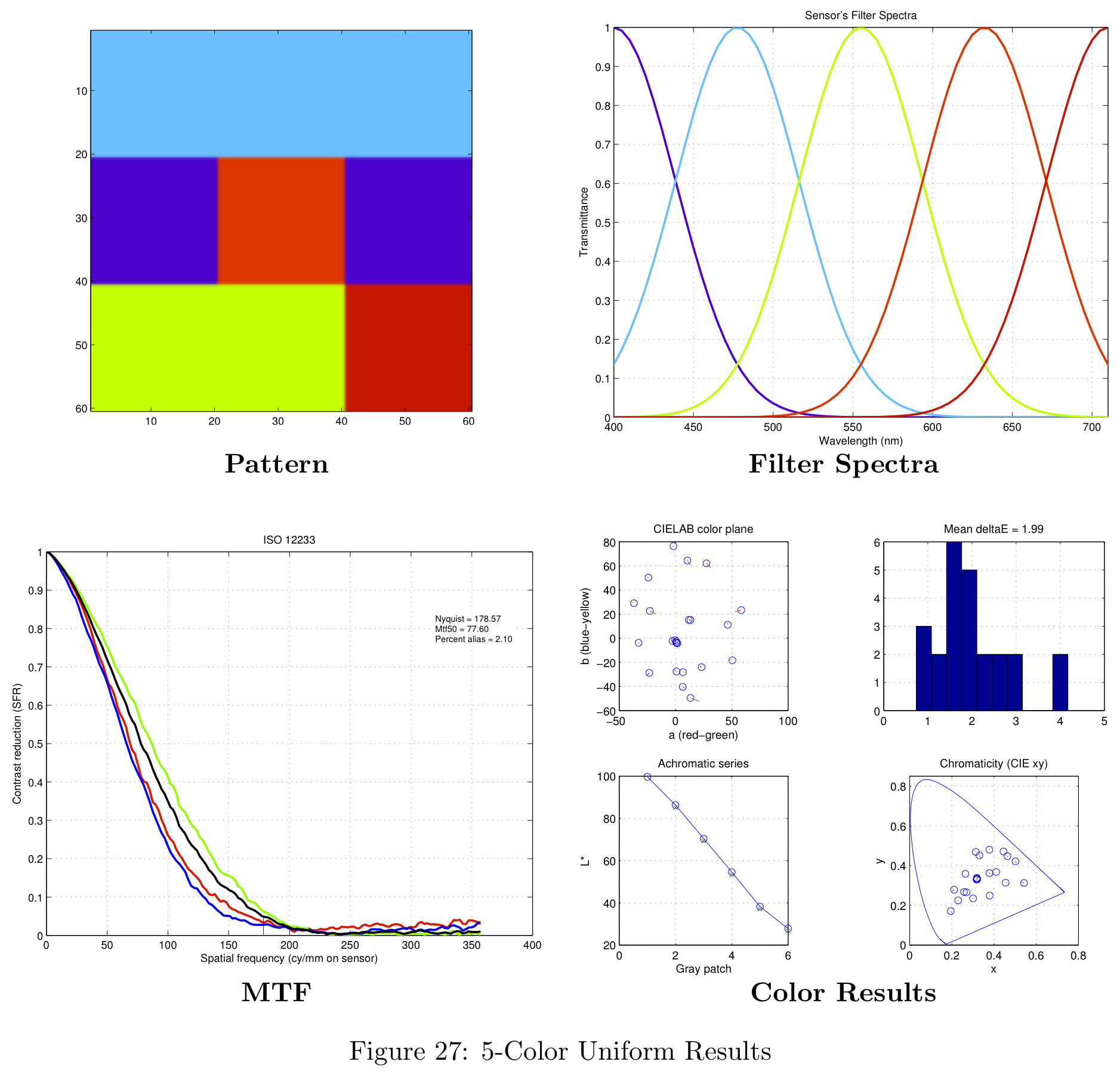
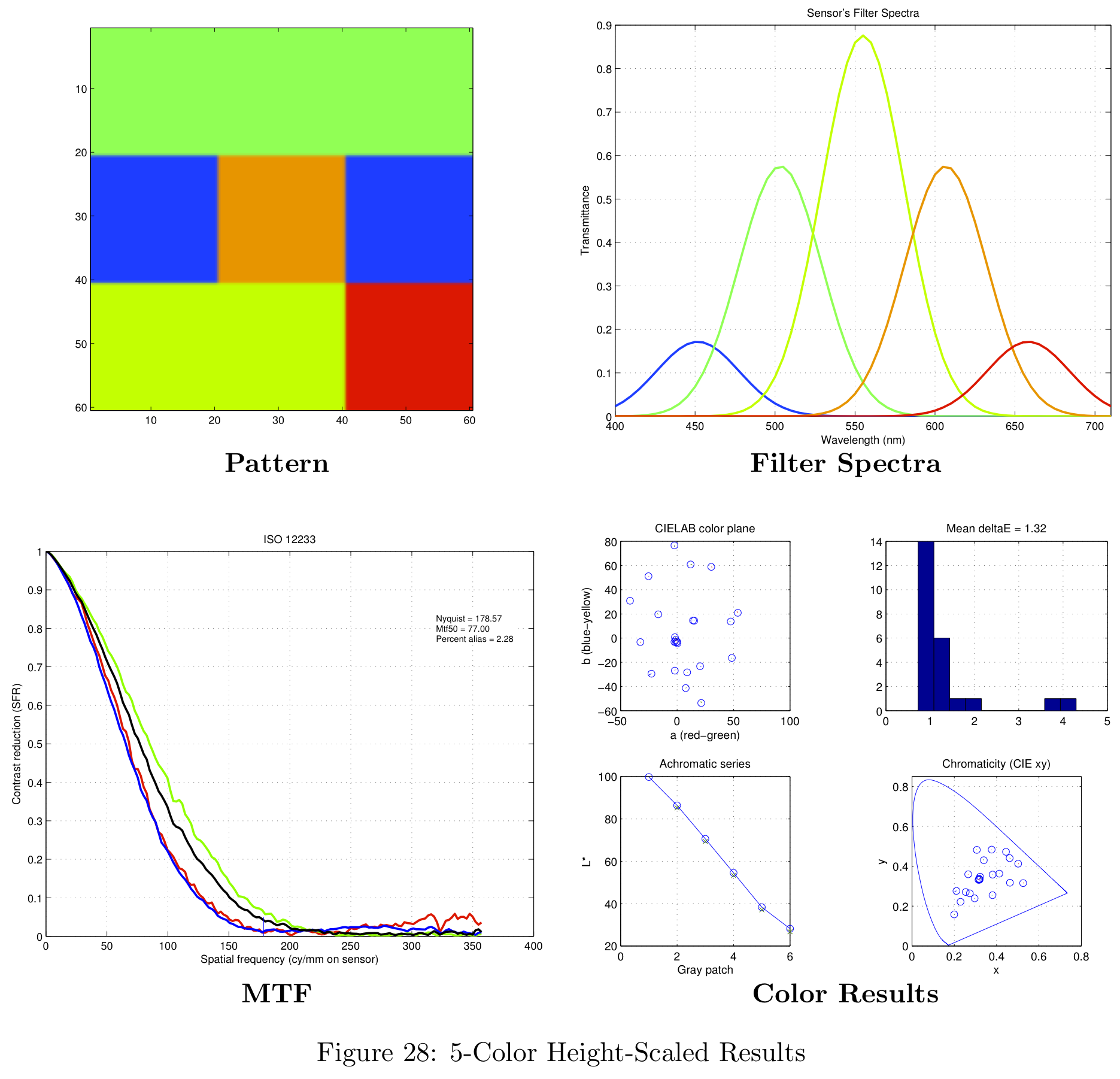
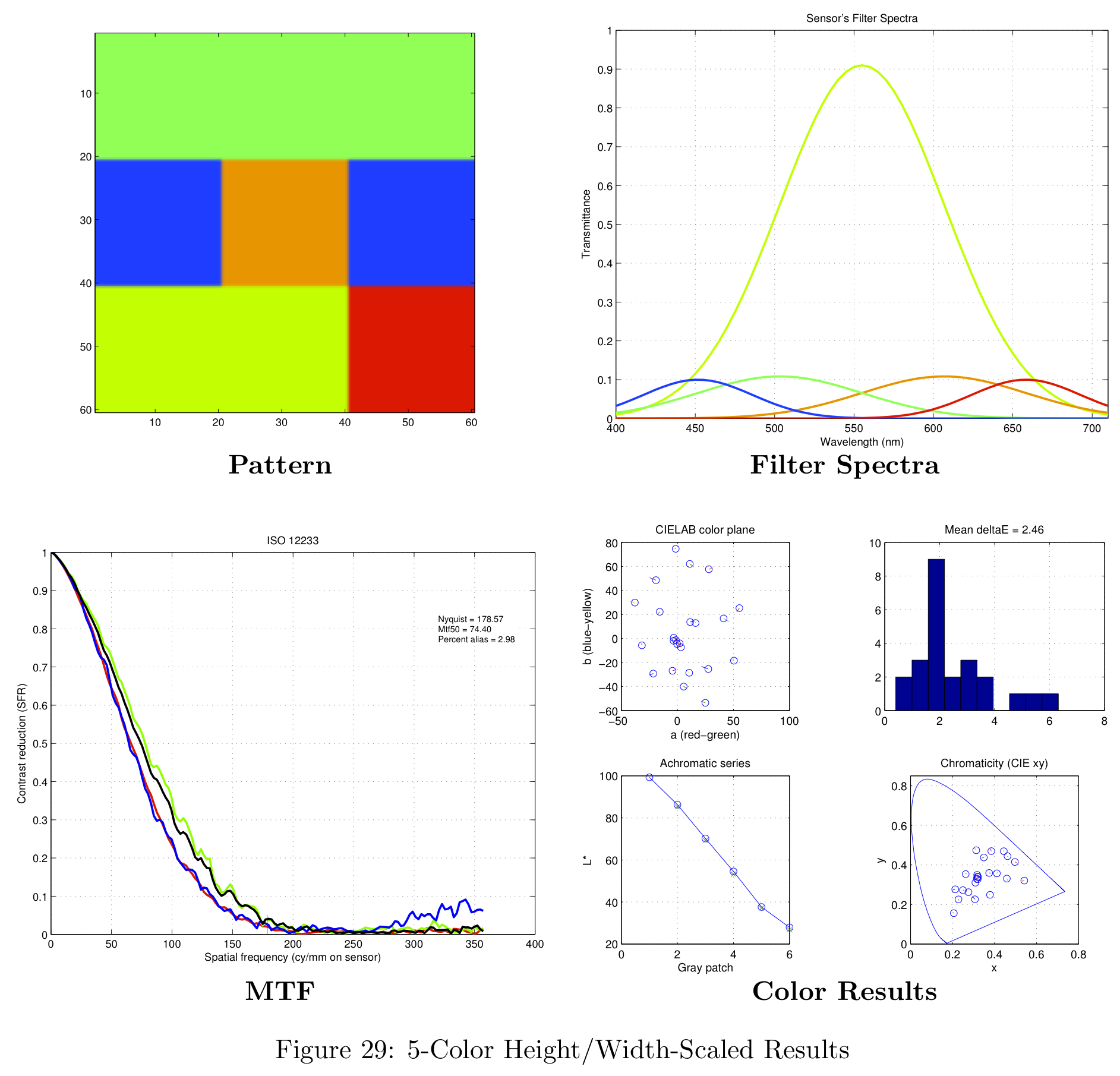
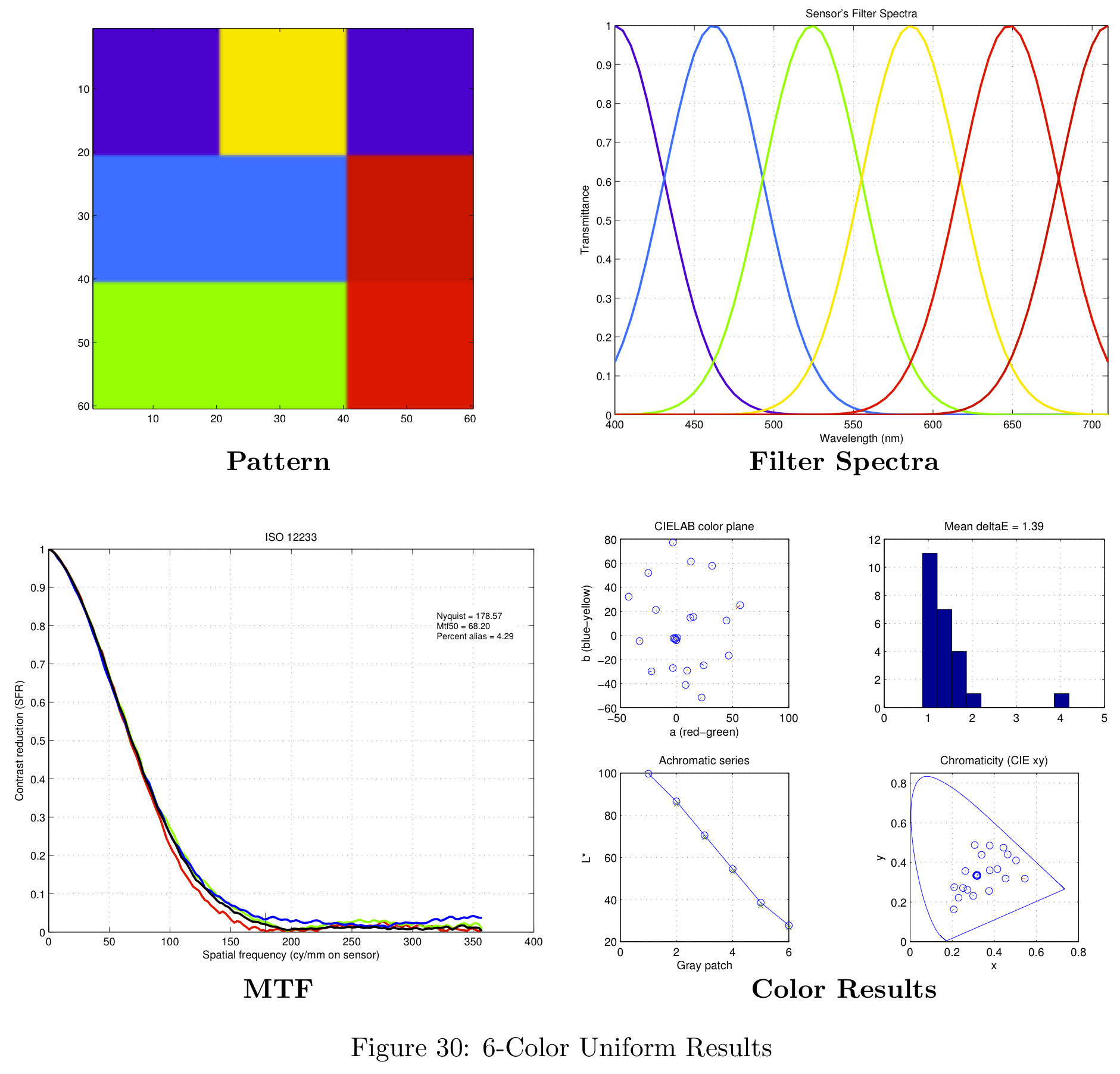
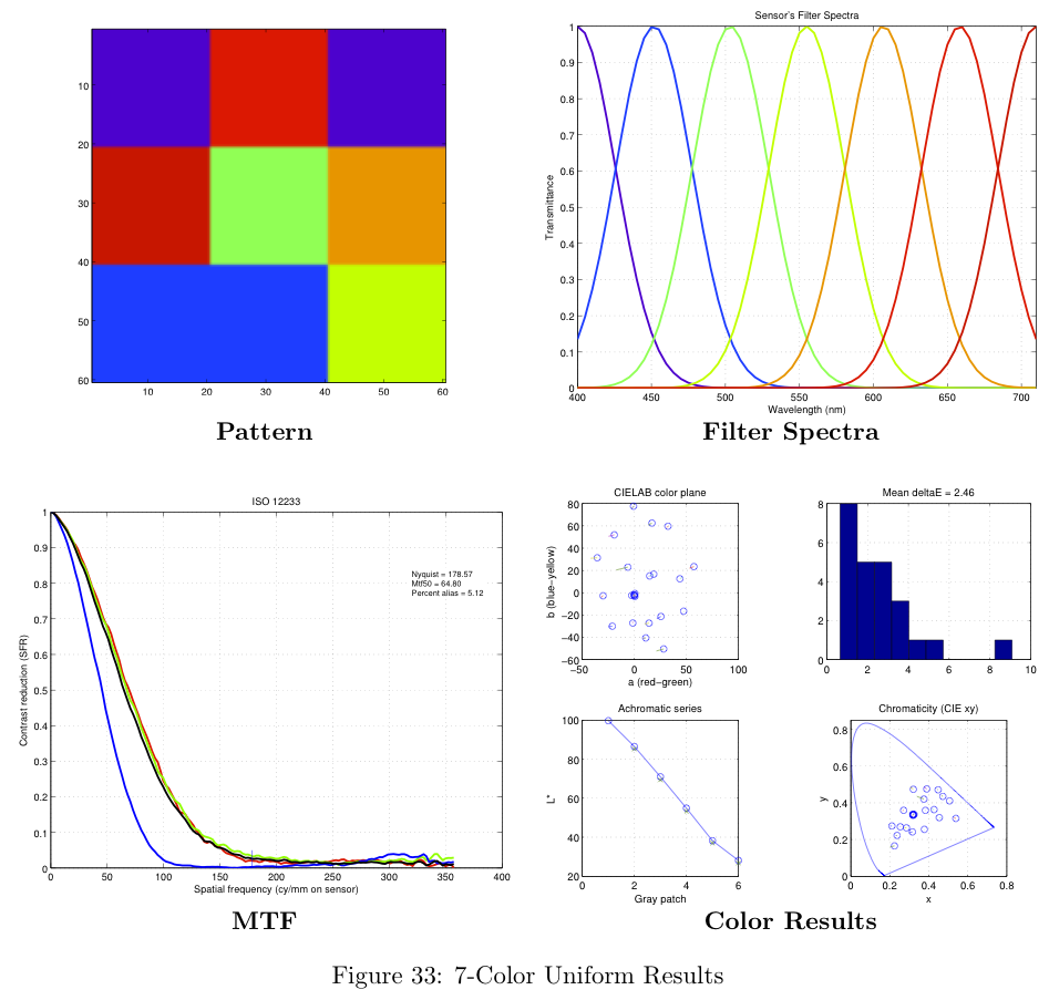
As a baseline, we created a set of sensors with uniform spacing between the filter centers, equal magnitudes for each filter, and equal filter widths. An example of this configuration's filter spectra is shown in Figure 10a.

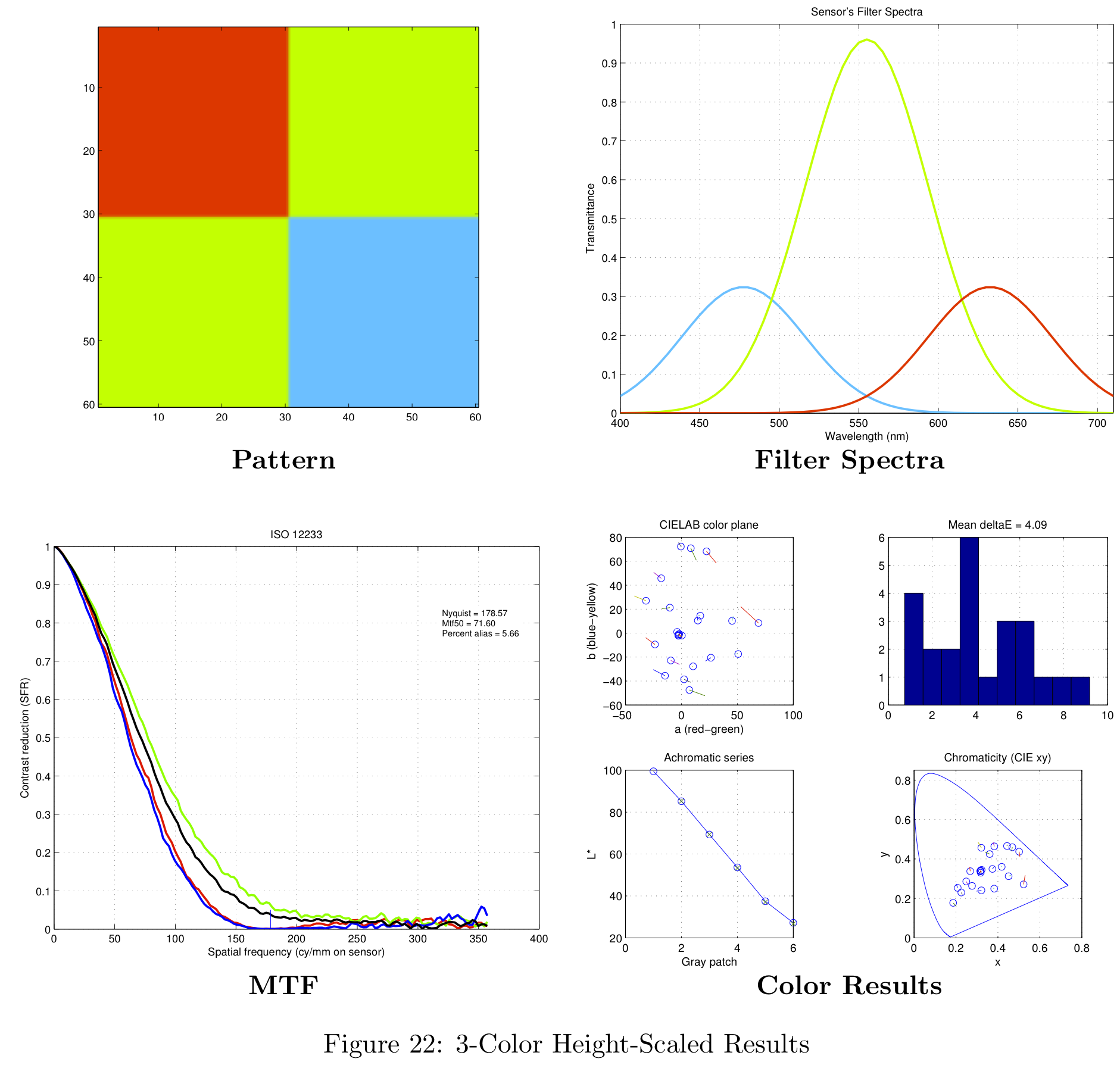
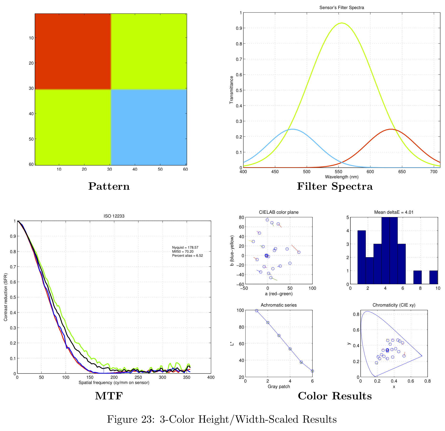
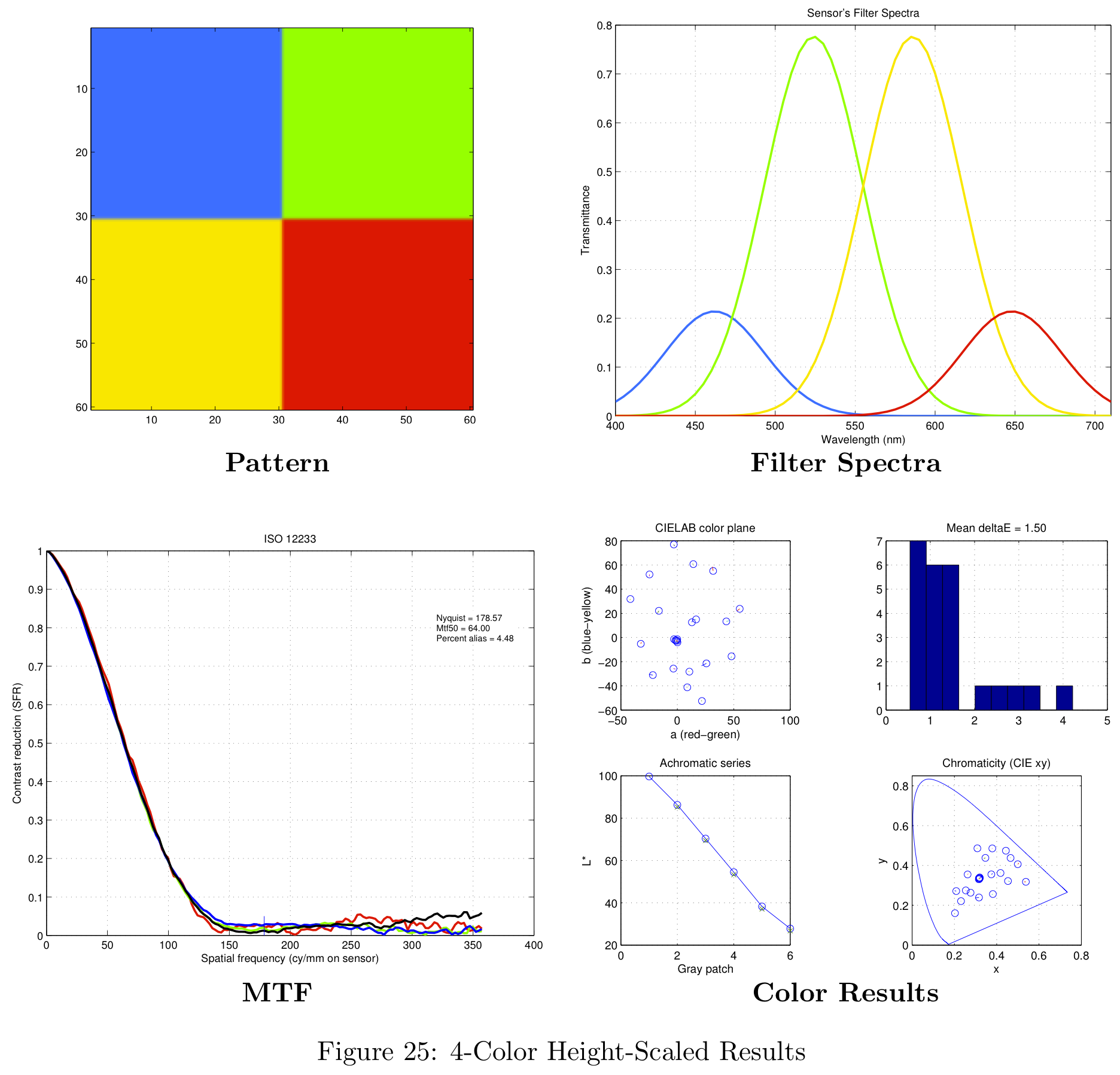
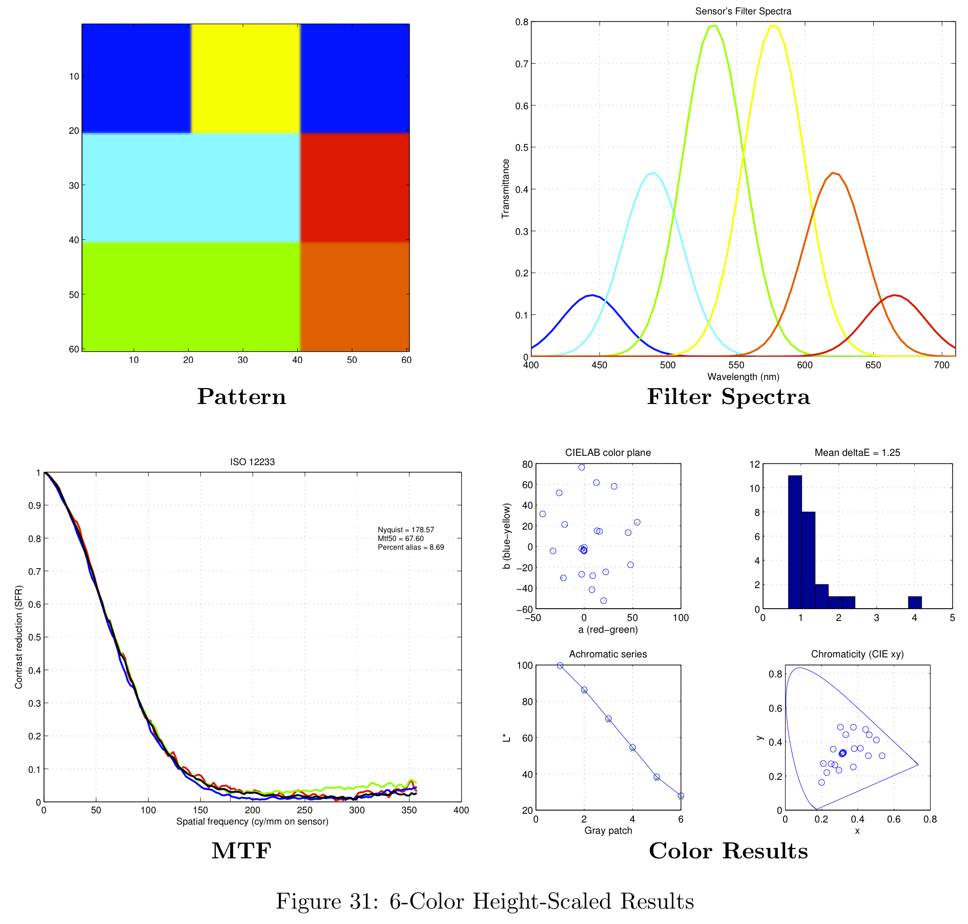
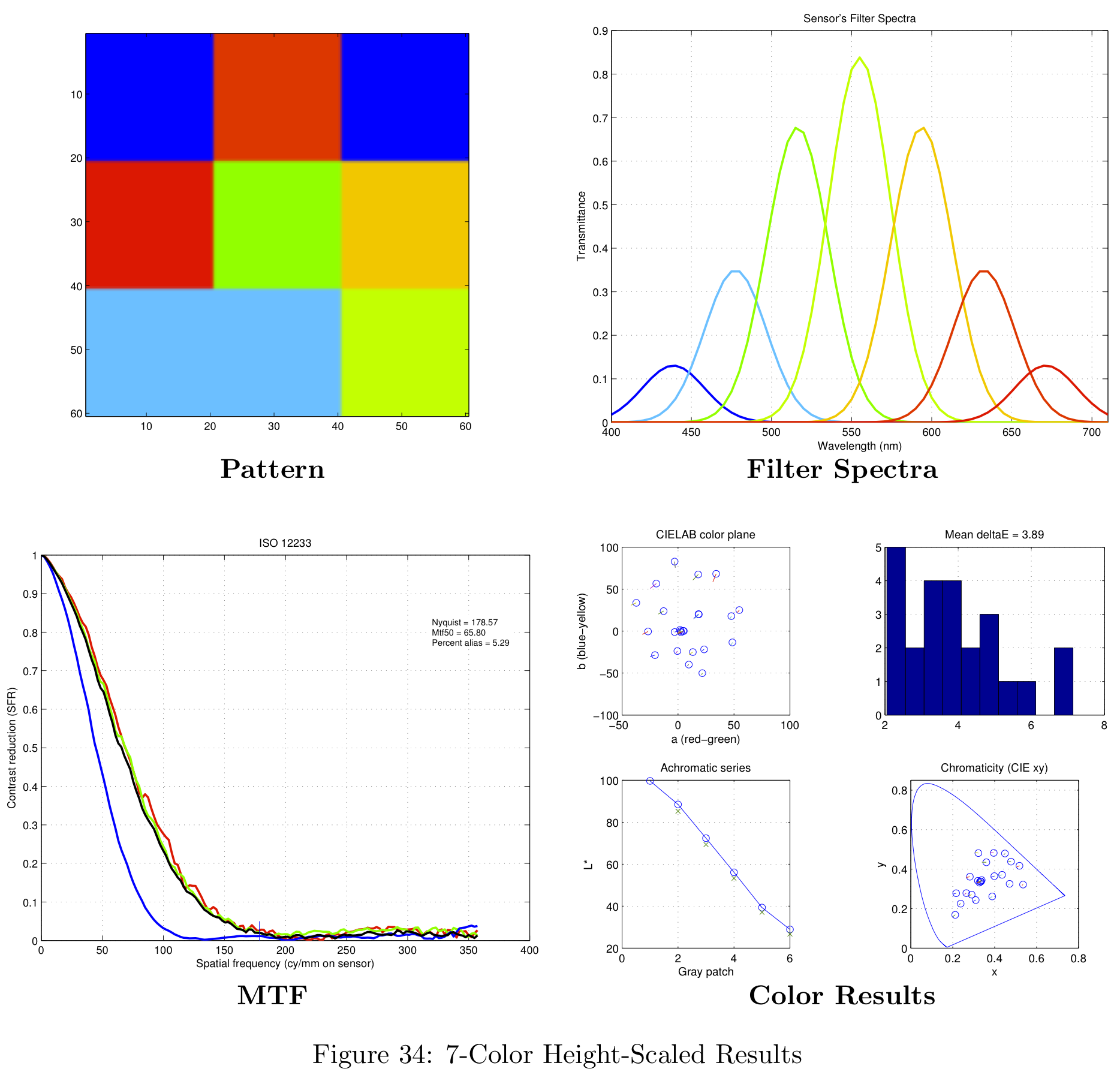
The next filter arrangement we tried was similar to the baseline design, but we allowed the magnitudes of the color filters to vary such that the overall response summed to a Gaussian. An example of this Height-Scaled configuration is shown in Figure 10b.

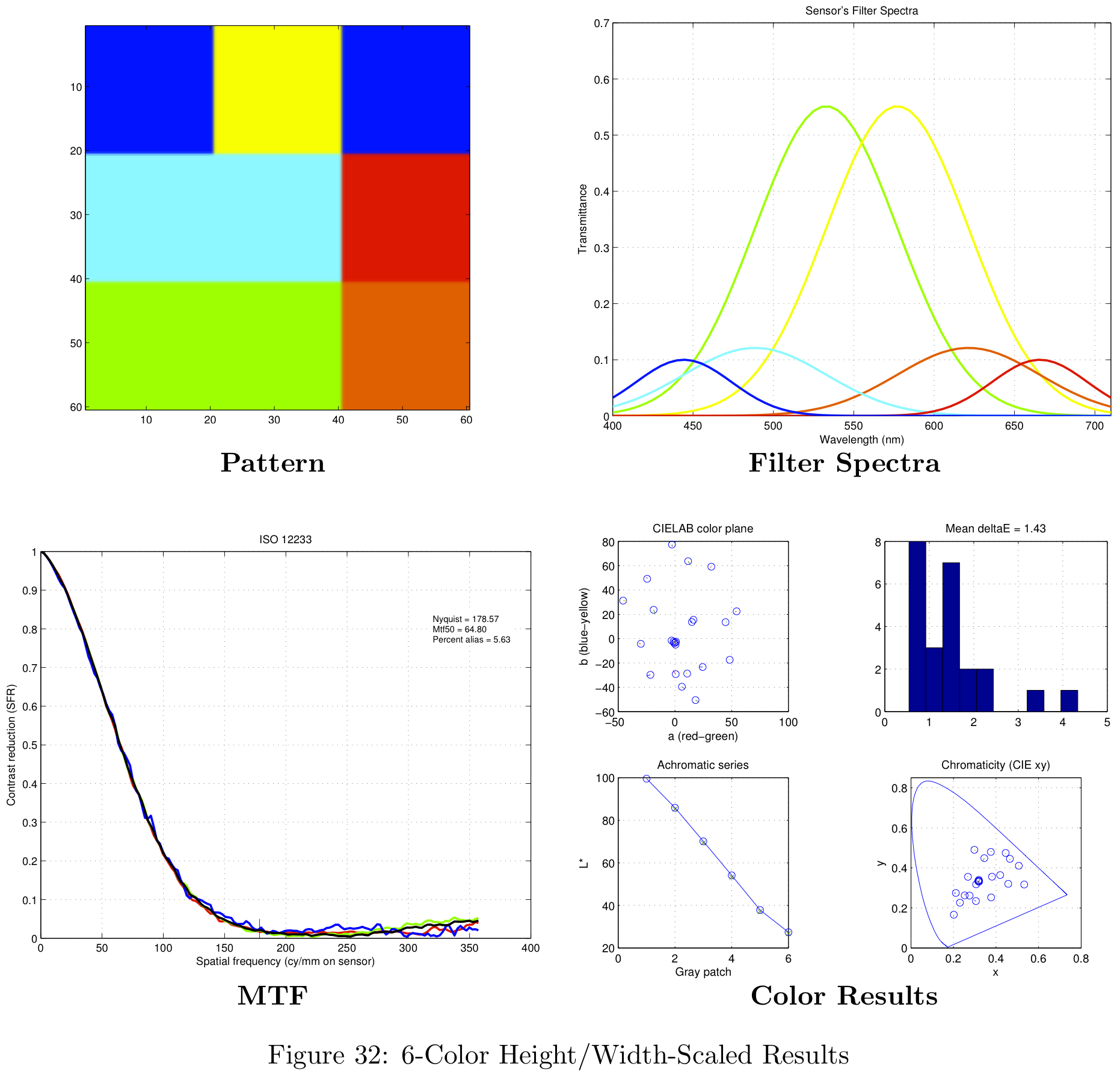
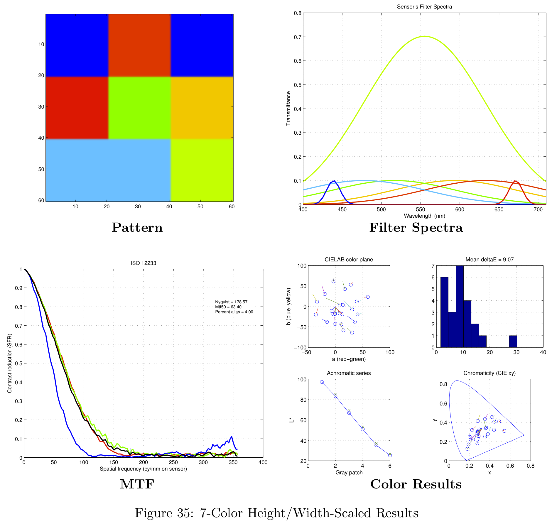
The last filter arrangement we tried is similar to both previous designs, but the filter magnitudes, filter widths, and filter centers were all allowed to scale to minimize the error between the sum of its spectral responses and a Gaussian.

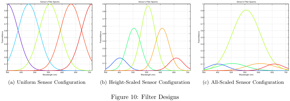
The All-Scaled approach (Figure 10c) conforms well to our Gaussian design rule, but the design is still sub-optimal. The center wavelengths are over emphasized, while the wavelengths at the extremes are under represented. Clearly additional design rules are required in order to optimize the tradeoffs between fitting to a Gaussian and the required frequency (wavelength) binning.

Defining the Spatial Pattern

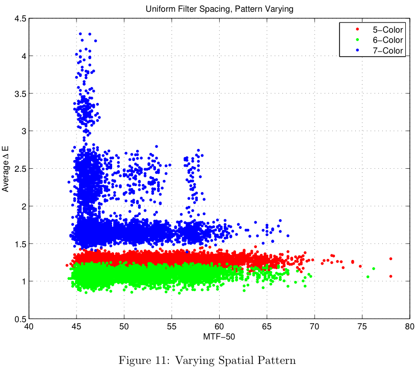
The first part of the design problem was to determine the specifications for the color filters. The second part of the design problem is to determine where the filters should be placed on the physical sensor grid. In order to determine the best physical layout, another brute-force simulation was run to iterate over a number of different design configurations. The results shown in Figure 11 were taken from a simulation with 5000 different sensor configurations. Each of the simulations was run with color filters satisfying the "Uniform" design criteria, mentioned in Theory-Based Simulation section.

Results

In this section we describe the results that were generated by using the methods of the previous section.

Defining Color Filters - Brute Force Results

The parameters that were used for the simulation are shown in the following table.

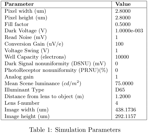
Figure 12 shows the results that were generated for 3 to 7 color sensors. We can see that the distribution gets tighter as the number of colors increases and that the delta-E value seems to approach a limit at around 1. Note that in this figure, a lower delta-E is better and a higher MTF-50 is better, so that the theoretical optimal sensor will be in the bottom right corner.

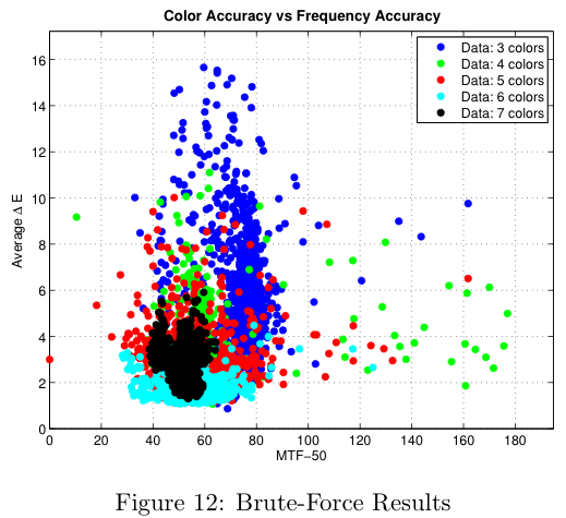
Plotting the sensor results on the same axis, we can see more clearly how the shape of the distribution changes as we increase the number of colors. For 3 colors, the delta-E values vary between 1 and 16, and the MTF-50 values between 30 and 160. The 4-color sensor gives lower variation in the delta-E values.

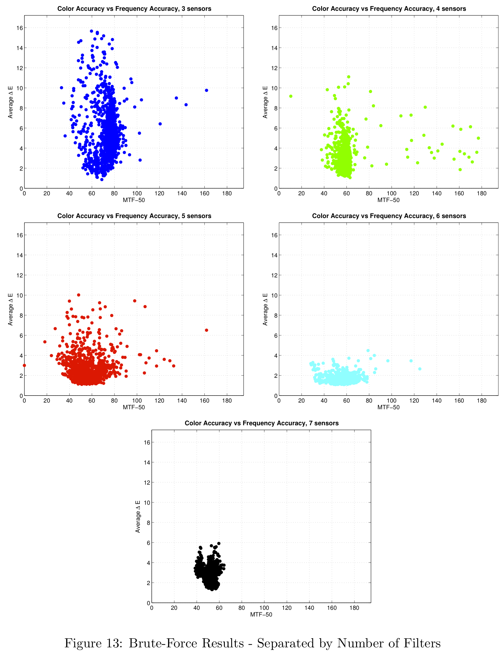
Moving to a 5-color sensor we expect to lose performance in frequency, since the size of the CFA is increased from 2x2 to 3x3. We know from Fourier theory that a larger patch in the spatial domain corresponds to a smaller bandwidth in frequency. This is exactly what happens as the 5-color distribution has a larger variance in the MTF-50 direction. The 6-color sensor has a lower variation in the delta-E direction than the 5-color version and the seven color case is interesting since it gives a very small variance in both color and resolution.

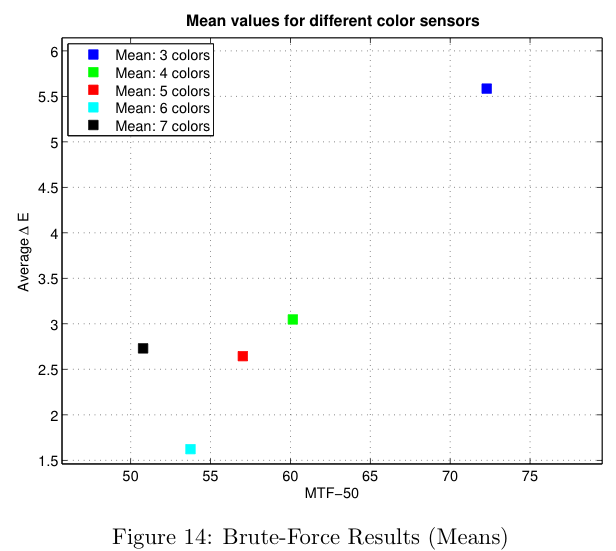
In the next figure the means of the different sensor simulations are shown. As expected, the spatial resolution decreases as we increase the number of colors. From 3 to 4 colors there is a large improvement in color, but also a large decrease in spatial resolution. It is interesting to note that the 7-color sensor is worse both in color and resolution than the 6-color sensor. Theoretically speaking, the more colors the sensor has, the better the color reproduction should be, so that this may be ascribed to the limitations placed on the simulation by the other parts of the imaging pipeline, such as the demosaicking and white balance routines.

A summary of the simulation results is shown in the next table. For each number of colors the delta-E and MTF-50 intervals that contain 90% of the samples are also calculated.

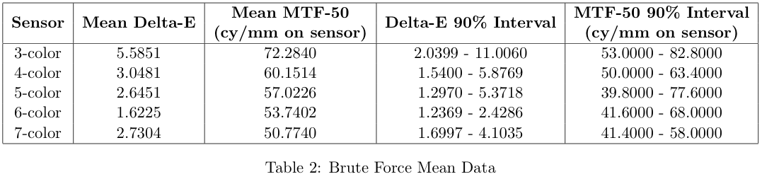
To get more insight about the different sensors that were simulated, the luminance noise was calculated for each of the simulations. The values used here are the means of the all the luminance noise values for the grey series of the color chart. The figures below show the simulation results again, with the color indicating the amount of luminance noise.

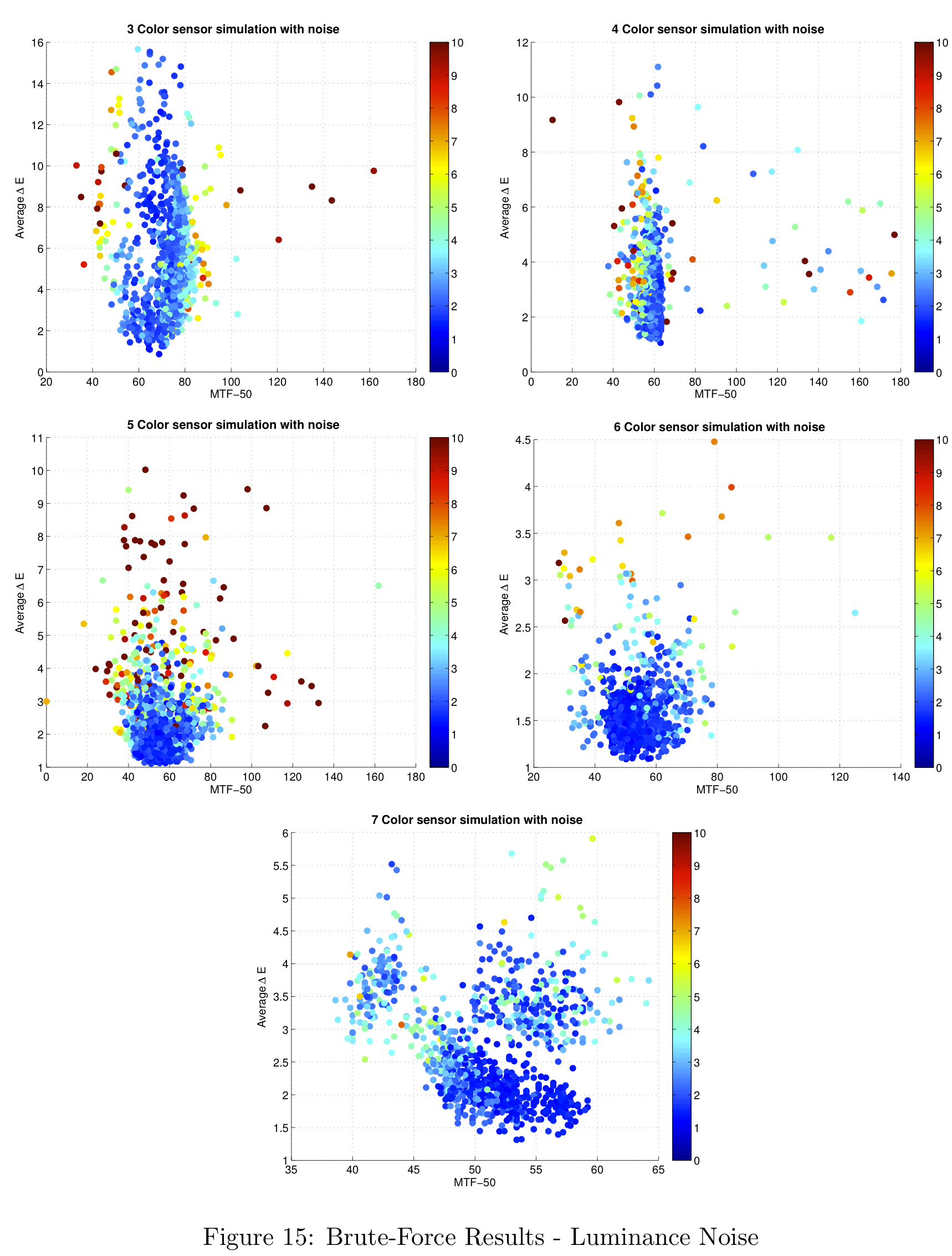
In general, the samples that are further from the mean have higher luminance noise, which motivates our choice of the mean as an indication of the performance of the sensor type as a whole.

Theory-Based Simulation Results

Figure 16 shows a summary of the theoretical results, and their comparison against the brute-force simulation results. Notice the number of color filters in each sensor configuration are grouped by different colors in the figure. For example, sensors with three color filters are shown in red. The different design methodologies (uniform, height-scaled, all-scaled) are represented with different symbols.

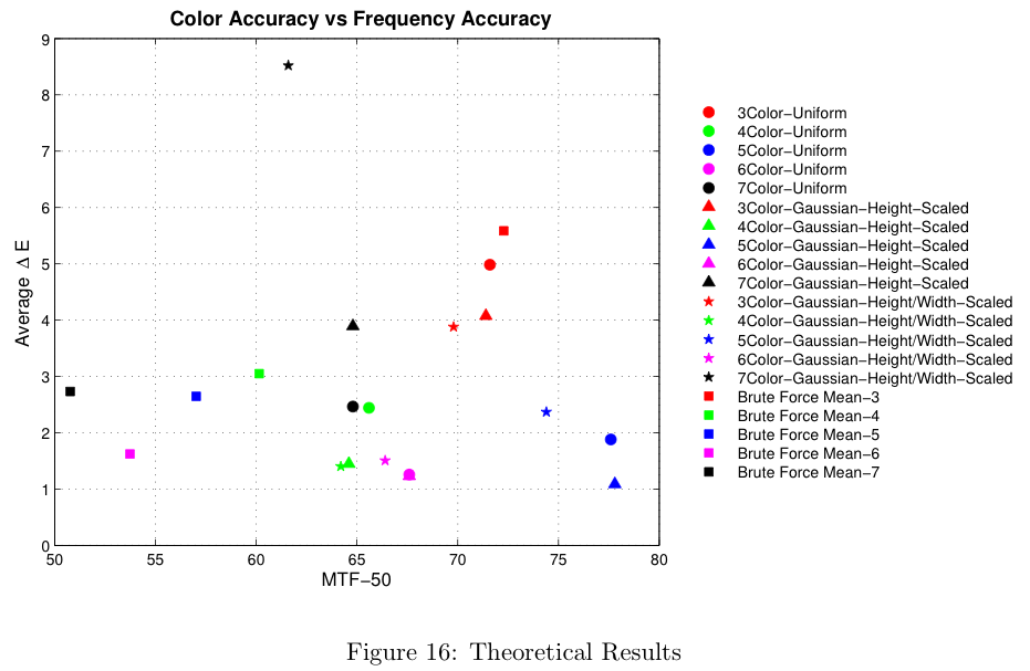
The results from the brute-force analysis are represented by box-shaped symbols. Notice the theoretical results typically exceed the performance of the mean in both color accuracy (lower average Delta-E) and spatial frequency response (MTF-50). The theoretical results do not, however, represent the best possible design.

Figure 16 represents a summary of the data collected. For more information on the data obtained with this analysis, please see the section in the Appendix on theoretical filter designs.

Spatial Pattern Results

The result of the spatial pattern analysis was a hand-picked sensor design based on the sensor's response shown in Figure 11 (section on Defining the Spatial Pattern). In this particular case, the "best" sensor chosen was the right-most data point for each of the distributions. The resulting patterns generated by this simulation are shown in Figure 17.

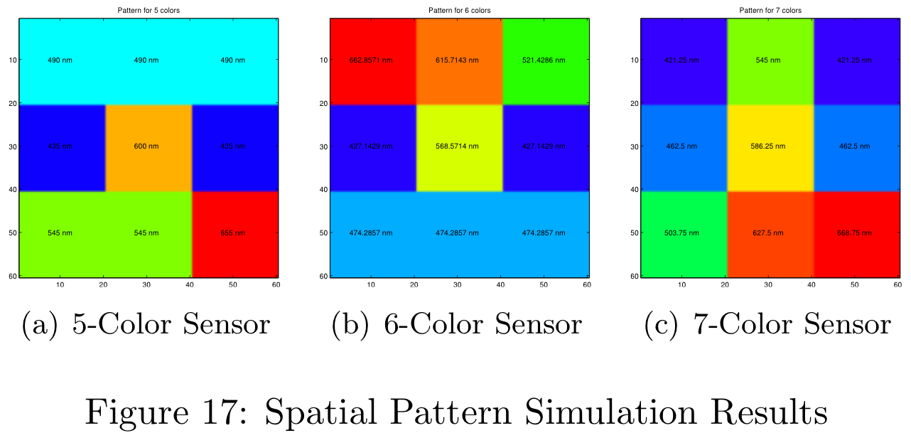
Each of these patterns were obtained for the uniform filter design. The simulation time for 1000 different patterns was approximately 4.5 hours on the 8-core machines in the CCRMA lab at Stanford. When simulating 5000 different patterns the simulation needed to run over night. Figure 17 is color-coded for the uniform filter design, but more information is available in the Appendix.

These color filter arrays are not necessarily the best possible choices for real-world images, they are simply the best choice given the Average Delta-E / MTF-50 tradeoff.

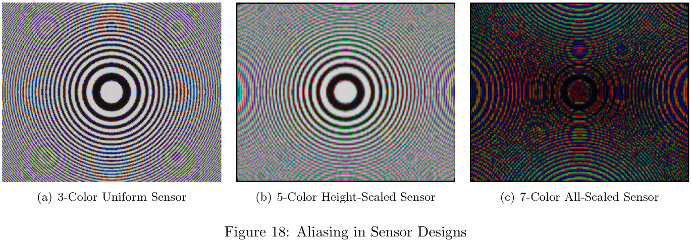
Aliasing

In order to get a reasonable visual representation of aliasing in our sensor designs, we modified the sceneCreate.m module within the ISET package. A Circular Zone Plate (CZP) scene was added and can be accessed from MATLAB with: scene = sceneCreate('zonePlate');. The CZP scene was chosen because Moire patterns are easily visible and produce some very interesting designs.

The aliasing effect resulting from each sensor design is clearly visible when analyzing the CZP scene, as shown in Figure 18. Notice there is substantially more aliasing in the 7-color design (Figure 18c) than in the 3-color design (Figure 18a).

"Real World" Results

Figure 19 shows the result of a simulated scene with two different filter configurations. The same two-dimensional pattern was used to capture both images.

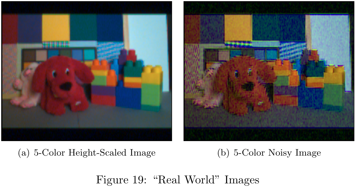
It is clear from these images that the filters chosen are critical to the final image quality. In order to see why the image quality is so poor, we can look at the filter spectra shown in Figure 20.

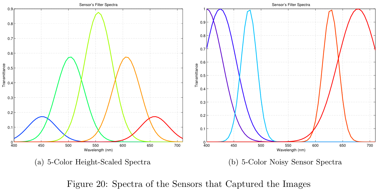
The spectra shown in Figure 20a represents the best theoretical results shown in Theoretical Results section. The image resulting from this design (Figure 19a) is of reasonable quality. The spectra shown in Figure 20b represents a sensor with poor results from the brute-force simulation. Notice the center of the spectrum is almost completely neglected. Since the human visual system is particularly sensitive to this middle-range of wavelengths, the final image (Figure 19b) is of poor quality.

Conclusion

It is clear from these results that both the filter choice and the placement within the filter array is critical in the production of high quality images. As we add additional color filters, we can see that the marginal color benefit resulting from adding a new filter decreases rapidly. The improvement to the average Delta-E value soon becomes smaller than the sensitivity of typical human perception and thus negates its benefit. The jump from three to four sensors offers a large improvement in color performance, but sacrifices a lot of spatial resolution.

The ISET simulation environment provided an effective means for comparing a large number of sensor configurations. Without a flexible simulation environment like ISET, this project would not have been possible. By grouping our MATLAB code into logical components, we were able to create a workflow which allowed us to define a single scene, a single set of optics and iterate through any number of sensor configurations.

When designing the individual color filters, it is important to choose a cost function properly. In the theoretical results section we can see the "all-scaled" design was under-constrained. By addition additional constraints to the design such as maximum filter width, minimum filter spacing, and minimum filter height we would likely have seen much better results.

Limitations of the Current Approach

There are a few limitations to the approach followed in this project and it is important to be aware of them when continuing this work. Firstly the brute force simulations take a very long time to compute, which makes it difficult to gather adequate statistics. For this reason it would be helpful if the ISET calculations can be sped up. Secondly, the ISET data structures seem to use more memory with each iteration, even when replacing the current objects with the new ones. This means the data has to be saved periodically and the structures need to be cleared after a fixed number of loops. Lastly, assuming a gaussian shape for each filter is not representative of manufacturing limitations, and if a more practical perspective is desired this method is less than ideal.

Future Work

This is a very large topic and there is much that can be done to continue this work. Using the simulation code that we have written as a base, one can explore many different aspects of the image pipeline that may affect the final choice of sensor. It would be good to simulate different shapes for the filter transmittance, and measure the effect of different illuminants. It would be particularly useful to upgrade the ISET tools to support other demosaicking and white-balancing techniques and see how they change the results with different numbers of colors.

Lastly, it would be interesting to set up a perceptual experiment to supplement the data from the simulation. For instance, if we use the sensor properties to generate pictures that people can rate, we can get a better sense of how different delta-E and MTF-50 values correspond to people's perception of image quality. For instance, we know that an MTF-50 value of 80 is better than 70, but if people can't tell the difference it doesn't matter and we should rather look at improving a different aspect of the sensor. After all, we shouldn't lose sight of the fact that cameras are designed to capture images for people, so that people are the ultimate judges of the quality of an image.

References

[1] P.B. Catrysse, B.A. Wandell, and A.E. Gamal. Comparative Analysis of Color Architectures for Image Sensors. Proceedings of the SPIE, 3650, 1999.

[2] J. Farrell, M. Parmar, P. Catrysse, and B. Wandell. Digital Camera Simulation. 2010.

[3] ISET Image Processing Pipeline, http://www.ImageVal.com, 2010.

[4] H.S. Malvar, L. He, and R. Cutler. High Quality Linear Interpolation for Demosaicking of Bayer-Patterned Color Images. 2004.

[5] J. Adams, K. Parulski, and K. Spaulding. Color Processing in Digital Cameras. IEEE, 0272-1732/98. 1998.

[6] http://www.perfectlum.com/manual/PressProof/images/images/colorchecker1.jpg. 2010.

[7] B. Wandell. Spatial Pattern Sensitivity (Lecture Presentation). 2010.

[8] Stephen H. Westin. http://www.graphics.cornell.edu/~westin/misc/res-chart.html. 2010.

[9] ISET - Calculating the System MTF Using ISO-12233 (Slanted Bar). http://www.imageval.com/public/Products/ISET/ApplicationNotes/SlantedBarMTF.pdf. 2010.