
In image processing, the appearance of a particular scene can be described as the combination of three factors: The reflectances in the scene, the scene illuminant (or lighting) and the device used for capturing the scene.
A scene pictured under different lightings can show considerable color differences. The human visual system is able to correct for this to a large extent, so that an object viewed under daylight looks similar when it is viewed under a lightbulb, for example. However, when a camera is used to take pictures of the object under the two illuminants, the differences can become very apparent.
The art of color balancing deals with correcting for these differences. Many different types of color balancing algorithms have been developed and they vary greatly in their complexity. An example of a simple algorithm is the gray world algorithm1, where the RGB components of an image are scaled to have the same mean value. Examples of more sophisticated algorithms are neural networks2 and Retinex3 methods.
In this project, color balancing was done on a scene consisting of a variable number of reflectances illuminated by tungsten light by finding a matrix which, when multiplied with each reflectance, gave the best average fit to what the reflectances would look like under D65 light. After having determined the matrix from this set of "training" reflectances, the matrix was then tested on a separate "testing" reflectance. The effects of altering the size of the training set were examined, as well as the effect of adding noise to the training set and performing the matrix fitting in XYZ or Lab space.
A Matlab application was designed to aid with the experiment as shown below.
The application works as follows: The user chooses the actual scene lighting in the "light" drop-down menu and an ideal light from the drop-down menu below. Typically these are tungsten and D65 lighting, respectively. Then a set of training reflectances is chosen, either by specifying a number of reflectances and then having the application randomly choose which ones to use, or by manually choosing each reflectance. A test reflectance is also chosen in the drop-down box on the right.
The option is also given to do the matrix estimation in Lab or XYZ space and to add noise to the reflectance set. Both of these options will be explained in better detail later, but to begin with, we assume that the simplest case of no noise and matrix estimation in XYZ space has been chosen. The parameters for the matrix estimation will then be as follows:
The XYZ values of a reflectance Ri under each lighting can then be calculated by the formulas XYZi-actual = RiT*Lactual*XYZconv and XYZi-ideal = RiT*Lideal*XYZconv.
To display the resulting vector, it is subsequently converted to RGB by multiplying with the sRGB matrix. The matrix XYZconv*sRGBT can be thought of as a device matrix, converting to the RGB values of a standard display.
We now want to find a 3x3 color balancing matrix CBM such that XYZi-balanced = CBM*XYZi-actual gives, on average, a reasonably good approximation for XYZi-ideal for all the reflectances. This can be done by defining XYZall-actual = [ XYZ1-actual XYZ2-actual ... XYZm-actual] and XYZall-ideal = [ XYZ1-ideal XYZ2-ideal ... XYZm-ideal ] and defining the color balancing matrix by CBM = XYZall-ideal*(XYZall-actualT*(XYZall-actual*XYZall-actualT)-1), which should give the minimum square error in the estimate. The resulting matrix is then used to color balance the test reflectance in the same way: XYZtest-balanced = CBM*XYZtest-actual. The color balancing matrix is shown at the bottom of the Matlab application.
To estimate how closely the result of our color balancing resembles the ideal reflectance, we convert both XYZi-balanced and XYZi-ideal to Lab space (the reference white point is the white patch of the Macbeth color checker under ideal light) and find the Euclidean distance between the two vectors, giving a ΔE value. The resulting ΔE values for the training set and the test reflectance are shown right below the corresponding color images in the Matlab application.
An interesting topic that comes into mind is whether better results (i.e. lower ΔE values) would be obtained by creating our conversion matrix in the Lab space, i.e. if we convert each XYZi-actual and XYZi-ideal to the corresponding Lab values Labi-actual and Labi-ideal and find the matrix that most efficiently converts the former to the latter, just as described above for the XYZ values. This gives us a color balanced vector Labi-balanced which can then be converted back to XYZ space and subsequently displayed. To help visualize the two different methods, the below figure is helpful:
![]()
Another point of interest is what effect, if any, it has to increase the number of reflectances in our training set, i.e. to increase m. On one hand, one might argue that by using more reflectances to create our color balancing matrix, we are "spanning" a larger fraction of all possible colors, thus doing better on average for a random test reflectance. On the other hand, by trying to fit a linear transformation to more reflectance vectors, the precision of each transformation will be worse.
Finally, it is interesting to examine the effects of adding noise to the reflectance vectors before the color balancing is done. This could be viewed as the effect of using a set of known reference colors in an image (such as a Macbeth color checker) to determine the appropriate color balancing method, but unbeknownst to the user, the reference colors have become smudged and tainted over time and thus would not resemble their ideal counterparts even under the appropriate light, such as D65.
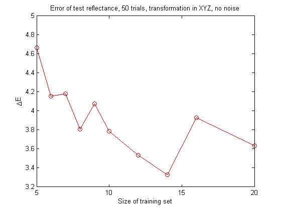
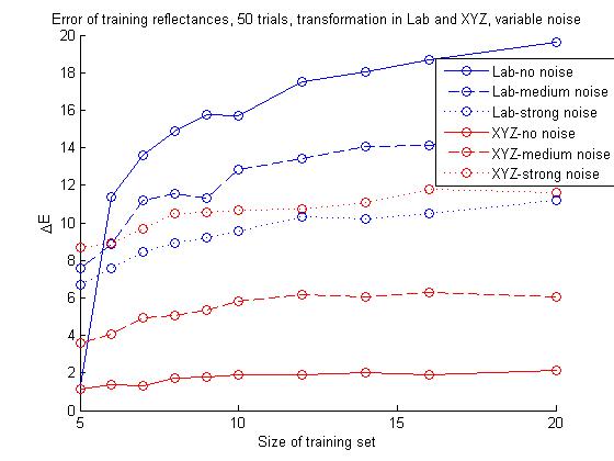
We begin with examining the effect of increasing the number of reflectances in our training set, while doing our linear transformation in XYZ space with no noise. The color balancing matrix was generated with a training set size of 5, 6, 7, 8, 9, 10, 12, 14, 16 and 20 reflectances and the resulting ΔE value for the training set and for the test reflectance recorded. This was done 50 times for each set size and the average values plotted.
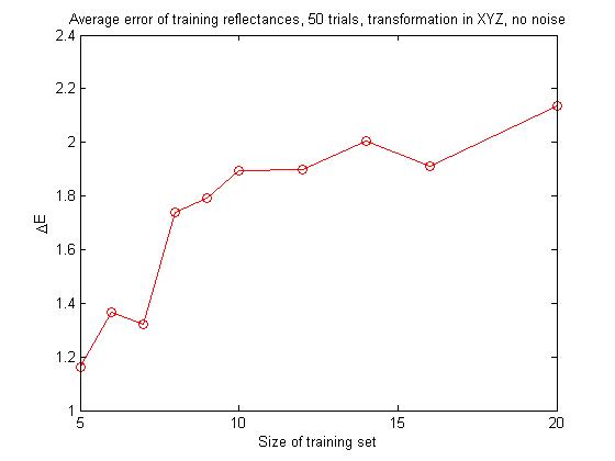
The upper plot shows the average ΔE value for the training set. The plot seem to show that as the number of training reflectances increases, the average ΔE value for the training set increases, indicating that as we try to fit the matrix transformation to more reflectances, the fit for each reflectance becomes worse on average.
The lower plot shows that as we use a larger range of reflectances to create the color balancing matrix, it does on average a better job of color balancing a new test reflectance, which makes intuitive sense.
As described above, here we are interested in whether we achieve lower values of ΔE by doing a linear transformation in XYZ space and comparing the Lab value of the result to the Lab value of the ideal reference, or if it is better to convert the reflectance values first to Lab space and do the best linear transformation there. As before, 50 tests were performed for training sets with 5, 6, 7, 8, 9, 10, 12, 14, 16 and 20 reflectances, but this time the matrix estimation was done in Lab space. The results for the training set (upper plot) and the test reflectance (lower plot) are shown below, along with the XYZ values from before for comparison.
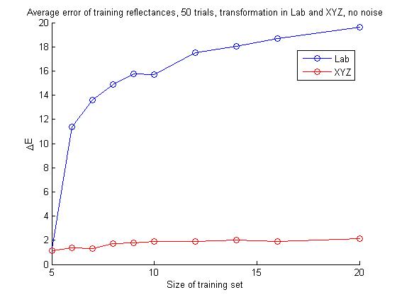
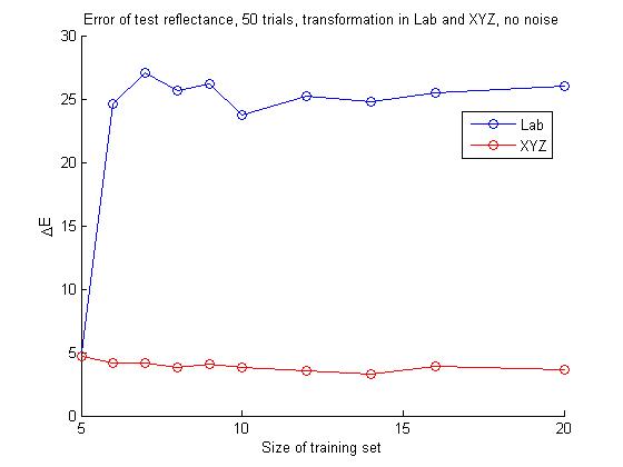
The plots indicate that constructing the color balancing matrix in XYZ space gives much better results than in Lab space, whether we are looking at the training set or the test reflectance. This seems somewhat counterintuitive, since the matrix estimation in Lab space is designed to produce the matrix which gives the smallest ΔE between Laball-actual and Laball-ideal. However, one must be careful comparing the two approaches, since the conversion between XYZ space and Lab space is nonlinear, and therefore constructing the color balancing matrix in XYZ space and then converting to Lab space is a nonlinear transform, seen from Lab space. Another way to look at this is that if we create the matrix in Lab space, we have already "locked in" a certain amount of error between the measured vectors and the target vectors in XYZ space, and therefore end up with a larger error. Furthermore, the error for the balancing of the test reflectance gets stronger as we train with more reflectances in Lab space, which seems somewhat counterintuitive. These results seem to indicate that creating the color balancing matrix in Lab space in general does not produce good results.
Another point of interest is to see what happens when we add noise to the reflectances. As described above, this can be viewed as using something akin to a Macbeth color checker in an image to get a reference for color balancing, but the color checker being dirty, worn out or otherwise damaged. The below image show the results of the same color balancing methods as before, but this time with added Poisson noise. The top image shows results for the training set with no noise, medium strength noise and strong noise. The bottom image shows the same for the test reflectance. The definition of noise strength was somewhat arbitrary, medium noise was defined as having standard deviation equal to 5% of the average value of the average reflectance and strong noise as having variance 10% of that same average value. These values are not significant in themselves, since we are only interested in seeing the trends in color balancing effectiveness as the noise gets stronger.
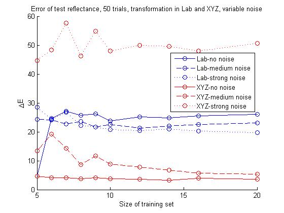
The plots show that the results of the color balancing gets worse as the noise gets stronger, and that the matrix calculation in XYZ is very sensitive to noise effects. Strangely, the Lab method seems to give slightly better results with stronger noise, but nonacceptable nonetheless. In fact, with strong noise, the Lab calculation becomes preferable to the XYZ calculation when balancing the test reflectance, since the XYZ method starts yielding such high error values that it can almost be viewed as useless.
One way of getting a sense of the variability of the color balancing matrix is to see where the white point maps for each estimate. This is done in the plots below, where each point represents the x, y values of the Macbeth white point, obtained by converting from tungsten to D65 with the matrix calculated in XYZ for all of the training set sizes. This was done for no noise, medium noise and strong noise, represented in the top, middle and bottom images, respectively.
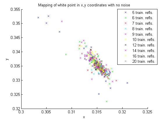
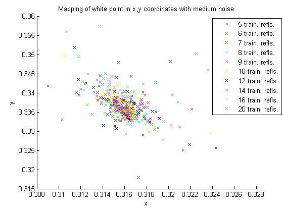
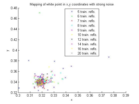
The plots seem to show two trends. First, as noise gets stronger, the points get more spread out. Second, this behavior seems to be more extreme for small training sets.
In this project, we have examined a relatively simple color balancing algorithm - finding the linear transformation that gives the least squares fit of a set of training reflectances to their values under ideal conditions. We have examined the effect of the training set size, the effect of noise and whether it is better to perform the least squares fit in XYZ space or in Lab space. The conclusions are as follows:
Furthermore, a Matlab application was developed to help with testing this method under various parameter settings.
Project presentation (this presentation contained a couple of errors in ΔE calculations, furthermore the scope of the testing was later increased from 5 training set sizes to 10 and from 15 trials to 50, so this presentation is a bit outdated. The information displayed on this page is more relevant).
Source code . (requires the ISET functions ieNotDefined.m, lab2xyz.m and vcXYZ2lab.m )