|
Simulation is a foundation of contemporary engineering design, without simulation it would often be impossible to predict the performance of modern devices using hand calculations. The ISET framework [2] simulates the entire imaging pipeline of a digital camera; this includes: input scene selection, optics formation, image sensors, pixel processing, and output display. Using the ISET framework, an engineer can visualize the final output of a simulated digital camera. Unfortunately, even simple shift-invariant or diffraction-limited optics can be quite computationally demanding. If the ray trace optics package is used to model a lens created with Zemax [6] or Code V [1], optics simulations can take several days when run on the host CPU.
Many algorithms, such as Fourier Transforms and affine transformations, used in image systems engineering are data-parallel algorithms. This form of parallelism is very easy to exploit on simple hardware. Each computational unit in a parallel computer can perform the same calculation on a different block of data. This model of computation is extremely well suited to the computational model and hardware resources available on a modern graphics processing unit (GPU). The application of GPU to data parallel problems allows for extremely high performance computing using commodity hardware. When ray trace optics are performed on an NVIDIA GeForce 9800 GX2 using the CUDA API[3], a small image (567 by 378 pixels) can be processed in under 18 minutes. The same image running on a 3.16 Intel Core 2 Duo microprocessor takes over a day to process, using the GPU for optics calculations results in an incredible 81x speed-up!
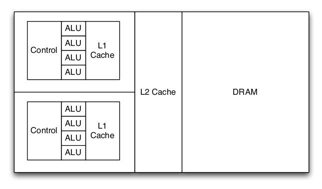
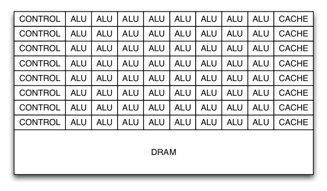
Modern graphics processors dedicate many more transistors to arithmetic processing units (ALU) than a conventional microprocessor. Conventional microprocessors dedicate a significant number of transistors to caches and complicated control structures in order to feed a small number of ALUs. This organization is beneficial to traditional desktop applications which are unable to exploit significant number of ALUs. Caches and complex control mechanisms are used to exploit the characteristics of desktop applications.
Graphics processors have traditionally been built with a fixed-function graphics pipeline used for rasterization. Programmability has been gradually added to the GPU: hardware transform and lighting, programmable vertex and pixel shaders, and most recently fully programmable hardware. Graphics applications take can advantage of a significant number of ALUs and have simple control structures. Most data is only used once, so caches are not helpful. The difference between a modern GPU and a modern CPU is shown in figure 1 and 2. The GPU has significantly more ALUs than the CPU; however, the large caches and complex control allows the CPU to execute a variety of code efficiently. The GPU only works well with certain types of applications.
To allow programmers to take advantage of the computation resources available on new graphics processors, NVIDIA has released the CUDA [10] (Compute Unified Device Architecture) on recent GPUs. All NVIDIA GPUs released after the G80 architecture (GeForce 8xxx series) have the ability to be programmed in C with custom-extensions to support execution on a GPU. The CUDA programming model assumes threads are working over an n-dimensional grid broken into smaller thread block. This model works well for image processing algorithms, which naturally fit on a two-dimensional grid.
The CUDA programming model also uses the concept of a kernel for functions that execute on the GPU. A CUDA program consists of several kernels that are executed serially. Within each kernel, hundreds of threads on the GPU perform calculation. The output of the first kernel becomes the input of second kernel. This model makes it simple to handle an arbitrary number of threads performing computation on the GPU. The extensions to the C programming language to support GPU computation require a separate compiler. This compiler, nvcc, is provided by NVIDIA for free and is required to compile programs interfacing with the GPU. The object files generated by nvcc can be linked with the native C/C++ compiler for the host platform. The ability to link to code compiled by nvcc makes it straightforward to call code on the GPU from traditional C code compiled by gcc on Linux / Mac OS X or Visual Studio on Microsoft Windows. The build process for GPU executables is a bit compiled, but the performance benefits far outweigh the complexity.
A potential downside of computation on the GPU is the disjoint address space. This means that memory addresses on the CPU are not usable on the GPU. Instead, data must be copied from the host CPUs memory onto the GPU. The copy between the host CPU and the GPU can become a bottleneck if the programmer is not careful. Large bulk transfers help alleviate the overhead of transfers from main memory to the GPU. If performed correctly, the disjoint address space is not much of an issue; however, too many small memory copies can significantly degrade performance. Other potential downsides of GPU computation include the lack of recursion and limited support for double-precision floating-point arithmetic on the GeForce 8 and 9 series. Lack of recursion not a problem; recursion can easily be converted into a loop. double-precision is an issue because MATLAB uses double precision floating-point values natively. In depth analysis would be needed to determine the impact of single-precision floating-point computation. Fortunately, the output of the GPU appears to be minimally affected by single-precision computation. Newer GPUs, starting from the GTX 2xx series, natively support doubleprecision in hardware. The Tesla series processors [5] are specifically designed for scientific computation; therefore,they natively support double-precision arithmetic.
In order to interface MATLAB with the CUDA GPU code, the MEX interface within MATLAB must be used. MEX allows MATLAB to call user-written functions in either C or FORTRAN. MEX wrappers allow the GPU code to interface with MATLAB. Other than interfacing with MATLAB, the MEX wrappers perform data-conversion for the GPU. MATLABs native data-type is double-precision while the GPU uses single-precision floating point. Therefore, the MEX wrapper must cast the double-precision values from MATLAB into single-precision values for the GPU and cast single-precision values from the GPU to double precision-values for MATLAB.
Both shift-invariant and diffraction-limited optics are based on convolution with an optical transfer function (OTF) for each wavelength in the input image. To explore the potential benefits of GPU technology in optics computation the diffraction and shift-invariant optics computations were first implemented on the GPU. Due to the lower computational complexity of the fast Fourier transform, I used Fourier Transforms instead of convolution. Therefore, the GPU code needs to take the two-dimensional Fourier transform of the input image, multiply the output element-wise with the OTF, and then take the inverse Fourier Transform.
Fortunately, NVIDIA provides the CUFFT library [4] of high performance Fourier Transforms. The CUFFT library is modeled after the popular open-source FFTW [7] library, which MATLAB internally uses. The downside of using the CUFFT is the different data organization for matrices between MATLAB and CUFFT. CUFFT assumes matrices are indexed in the row-major form (the convention used by the C programming language) while MATLAB assumes column-major (the convention used by FORTRAN). Simply stated, when a matrix is represented by an array MATLAB assumes the array is the concatenation of the columns while CUFFT assumes it is the concatenation of the rows. In order to avoid dealing with the indexing issues and increase the precision of the result, the input image is padded so that its both square and a power-of-two. The square matrix avoids issues with indexing while using matrix dimensions that are a power-of-two allows for a more accurate FFT algorithm.
|
The shift-invariant optics code is very simple; it copies the OTF to the GPU then performs the computation shown in algorithm 1.
 | (1) |
 | (2) |
|
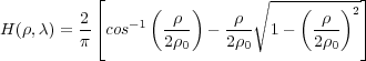
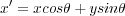
The diffraction-limited optics algorithm is shown in algorithm 2. In order to accelerate the computation of the diffraction-limited OTF calculation, OTF is computed on the GPU. The equations presented in Optical transfer function of a diffraction-limited system for polychromatic illumination [11] are used for the computation on the GPU. The equations presented in the paper are shown in equations (1) and (2). In the equations, ρ is the spatial frequency in polar coordinates and di is the distance between the aperature and the image detector plane. Equation (1) is only valid if ρ ≤ 2ρ0, otherwise H(ρ,λ) = 0.
The square root and arccosine calculations can be computed in a small-handful of cycles on the GPU while they take much longer on the host CPU. The difference computation time on both GPU and CPU dependent upon the design of the floating-point units. There is small amount of precision lost when the OTF is calculated on the GPU; however, the difference between the CPU and GPU computation is not visible.
The shift-invariant and diffraction-limited optics are minimally optimized; there are most likely significant opportunities to perform more computation on the GPU. That said, the run-time for shift-invariant and diffraction-limited optics is relatively short anyways (approximately two minutes on average) and the optics transform is not on the critical path.
The ray trace optics calculations are much more computationally demanding the shift-invariant point spread computations. Instead of performing a series of Fourier transforms, a series of wavelength-dependent point spread functions are applied to the image pixel by pixel. Each pixel is displaced according to a displacement field then blurred using a local point spread function. A benefit of using the ray trace optics package is that lens designed in a lens CAD program can used the ISET image processing pipeline. Lens designed in either Code V or Zemax can be used by ISET.
Without GPU acceleration, the ray trace optics package is extremely slow. Very small images (64 by 96 pixels) take over an hour on the fastest available machines. A reasonably sized image (567 by 378 pixels) takes over a day! Adding more CPUs to a system does not improve performance significantly; MATLAB is unable to efficiently take advantage of the additional processors. Future MATLAB releases will include the Parallel Computing Toolbox [9] to allow a programmer to use message-passing techniques exploit loop-level parallelism on a cluster or multiprocessor machine. Unfortunately, the Parallel Computing Toolbox only supports eight threads per host and requires cluster of computers for further scaling. The technology will still require modification to the program and the cost of additional software. Using a GPU is a much more cost-effective way of accelerating the ray trace code.
|
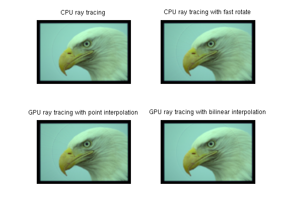
The ray trace optics algorithm is shown in algorithm 3 The loop iterates over all photon wavelengths, the height of the image, and all pixels. The inner loop iterates over every pixel in the image, computing a local point spread function then applying to the input. This calculation involves adding two-weighted point spread functions and rotating according the lens parameters. The rotated point spread is then interpolated to create the final point spread function. The point spread is then applied to the image through a simple summation. Partitioning ray trace computation for the GPU is essential, too little work and the run-time will be dominated by the overhead of transferring data to and from the GPU. Too much work will not fit on the GPU and the calculation will have to be divided into small blocks. For maximum speed-up, the entire inner loop is computed on the GPU. This is a natural partitioning because it allows one large transfer up to the GPU, lots of computation, then a small transfer back to the CPU. The inner loop partitioning also allows multiple GPUs to be potentially used; different GPUs could compute work on different wavelengths in parallel.
The GPU code for ray tracing code uses several kernels to perform calculations, the flow of data between kernels is shown in figure 3. These include weighted summation, image rotation (using point sampling or bilinear interpolation), image interpolation, reduction, summation, and scaling. All of the kernels except rotation and interpolation are very simple. The rotation and interpolation kernels are more complex for reasons of precision and performance. The connection of the kernels and host code is shown in figure().
 | (3) |
 | (4) |
 | (5) |
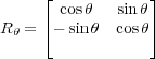
The host CPU code uses the MATLAB imrotate function; this function is not entirely documented so two versions of the rotation kernel were implemented in order to better match the output of the MATLAB function. The first version of the GPU rotation code uses a nearest point approximation. Each output pixel is calculated by computing the X/Y coordinates for the input pixel given the rotation angle. This is simply a multiplication by a rotation matrix, a simple linear transform. If the input pixel is outside the dimensions of the image, the output pixel is assigned zero (this corresponds to a rotation with crop); otherwise the value at the calculated coordinates is used. If the output coordinates have a fractional component, they are rounded to the nearest pixel. The nearest pixel rotation method is simple and computationally cheap, but leaves some small rotation artifacts stretching from the center of the image.
The first steps of the bilinear interpolation rotation are similar to the nearest point approximation. Instead of rounding the X/Y coordinates to the nearest pixel, the kernel uses bilinear interpolation among the four nearest neighbors. This method removes the rotation artifacts seen with the point approximation method but slightly blurs the overall image. It is also more computationally demanding due to the computational cost of bilinear interpolation. In particular, four more loads from memory must be performed for each pixel. GPUs do not have caches like a traditional processor so the cost of the additional loads has the potential to be quite significant. In practice, the run-time of ray tracing optics with the bilinear rotation kernel is approximately twenty-five percent greater than point approximation. If the overhead becomes significant, it is possible to use shared-memory in each GPU multiprocessor as a cache managed by software.
![tex(x,y) = (1 - α)(1 - β)T[i,j]+ α(1- β)T[i+ 1,j]+ β (1 - α)T[i,j + 1]+ αβT [i+ 1,j + 1]](project5x.png) | (6) |
 | (7) |
 | (8) |
 | (9) |
 | (10) |
The interpolation kernel uses special hardware on the GPU designed for handling textures when the graphics processor is used for rasterization. Equations (6) through (10) show the interpolation performed on the GPU. A MATLAB plugin performing rotation is available from [8]. The texturing hardware does not provide full single-precision accuracy but the accuracy appears good enough for the purposes of the optics ray trace code. Further analysis would be required to determine exactly how much precision is safely needed. Fortunately, the output of ray tracing clearly shows any significant computational errors that may have occurred because the output appears very wrong.
Data has to be explicitly boxed to use the proper formation for the interpolation hardware, but the computation is effectively free other than the cost of data manipulation. Within the GPU ray tracing code, the output from the rotation kernel must be transformed into texture in order to use the interpolation hardware. This is a relatively simple memory operation. Interpolation on the GPU also requires a grid a corresponding to the desired output texture size. The cost of creating an output grid is amortized by the fact that it can be repeatedly used during call to the GPU ray tracing code.
The ISET MATLAB code had to be slightly modified to support GPU computation. To support the shift-invariant and diffraction-limited optics, the opticsOTF.m file was slightly rearranged. Some of the computation that traditionally in the functions used to manipulate OTFs was hoisted into the opticsOTF.m file. This made it easier to calculate all of the parameters needed for the diffraction-limited optics without modifying a large number of files. In addition, cpu_filter, was added to model the computation performed on the GPU, gpu_filter, it was function to benchmark and debug the GPU code.
The ray trace code also required a small number of changes. In particular, the inner loop of the computation was replaced by the GPU computation function, gpu_bulk_rt. This required some minor code motion to compute the required parameters for the GPU function ahead of time. The ray tracing code benefits from some minor code clean by hand-applying loop-invariant code motion to remove calculations involving constant values from loops.
In order to evaluation the performance benefit of GPU computation within the ISET framework, the GPU code was run on three different test systems. The first test system was an Apple MacBook Pro. The laptop has a relatively low-end GPU, the NVIDIA GeForce 8600M GT. The 8600 M GT has 512 megabytes of memory attached to the GPU through a 128-bit wide interface. The chip can have up to 32 threads in flight. The second test system was a generic PC with a NVIDIA GeForce 9800 GT. The GeForce 9800 GT has 512 megabytes of memory attached to the GPU through a 256-bit wide interface. The 9800 GT can have 112 threads in flight. The final system has an NVIDIA GeForce 9800 GX2. The 9800 GX2 is based on the same ASIC as the 9800 GT; however, the memory interface is clocked at a higher frequency and 128 threads can be in flight. The second GPU on the GX2 card was not used.
| MacBook Pro | Generic Desktop 1 | Generic Desktop 2 | |
| Processor | T9300 | E6600 | E8500 |
| Frequency | 2.5 GHz | 2.4 GHz | 3.16 GHz |
| L2 Cache | 6 MB | 4 MB | 6 MB |
| Memory | 2 GB | 4 GB | 8 GB |
| GPU | GeForce 8600M GT | GeForce 9800 GT | GeForce 9800 GX2 |
| GPU Memory | 512 MB | 512 MB | 512 MB |
| GPU Memory Frequency | 700 MHz | 900 MHz | 1 GHz |
| GPU Bus Width | 128 bit | 256 bit | 256 bit |
| GPU Threads | 32 | 112 | 128 |
| MATLAB Version | 2008b | 2008b | 2007a |
| OS | OS X 10.5.6 | Linux 2.6.28.19 | Linux 2.6.28.19 |
 | (11) |
 | (12) |
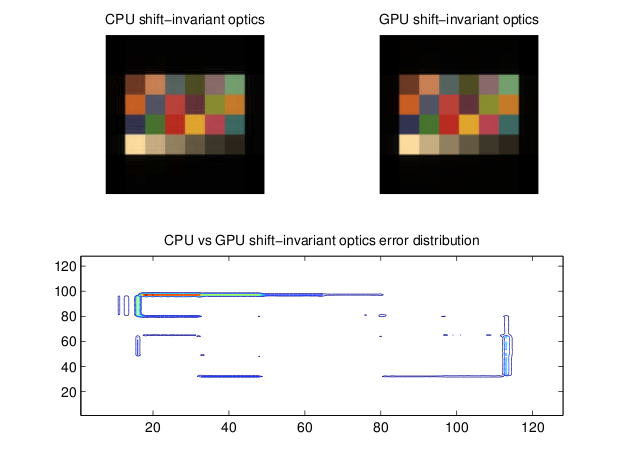
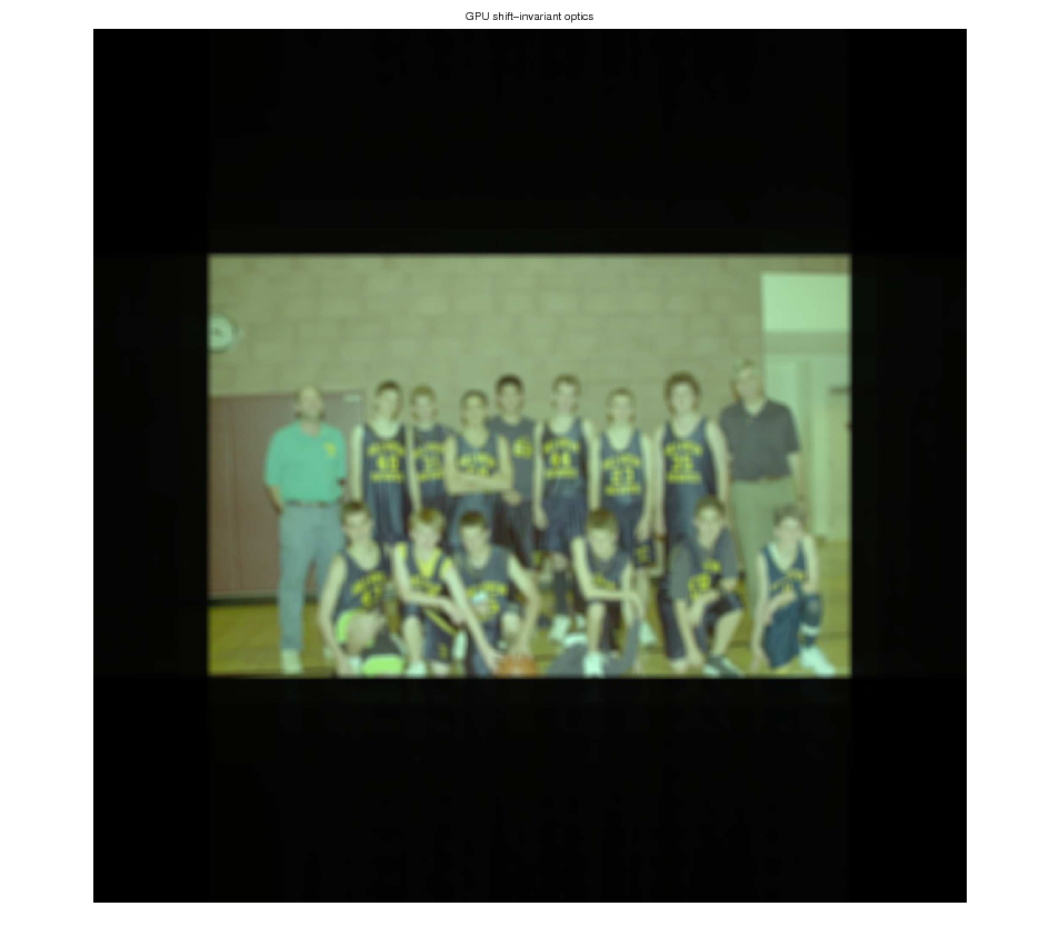
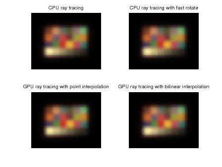
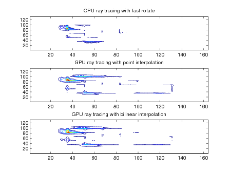
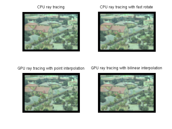
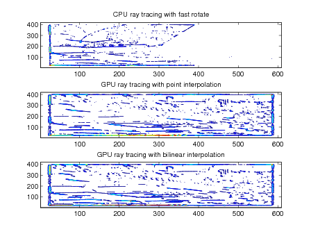
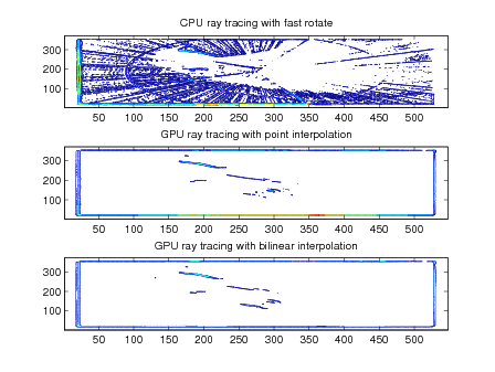
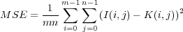
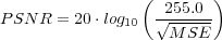
Shift-invariant, diffraction-limited, and ray trace optics were evaluated using mean squared error and peak signal-to-noise. The equations for PSNR is shown in equation (12) and MSE is shown in equation (11). Output images after the optics computation are also included in the results section; larger versions are available in the appendix. Contour plots of the squared-error between optics calculated on the GPU and CPU help identify regions where GPU computation significantly deviates from the CPU calculation.
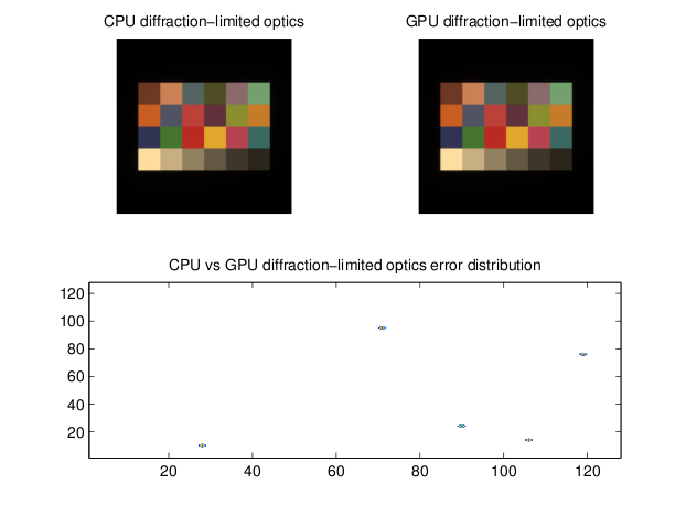
In general, the shift-invariant optics calculation has both good performance and accuracy. The PSNR is quite good for both the Macbeth chart and basketball team. Some occurs along edges in the two-images. This is probably causes by the difference between the single-precision calculations performed on the GPU and MATLAB’s native double-precision calculations.
The Macbeth D50 chart runs quickly on the CPU, so performance numbers were not recorded. It was only used to compare the algorithm running on the GPU and CPU. The basketball team sees a reasonable speed-up on the GPU; however, much of the remaining run-time is dominated by serial code that runs on the CPU.
|
|
|
|
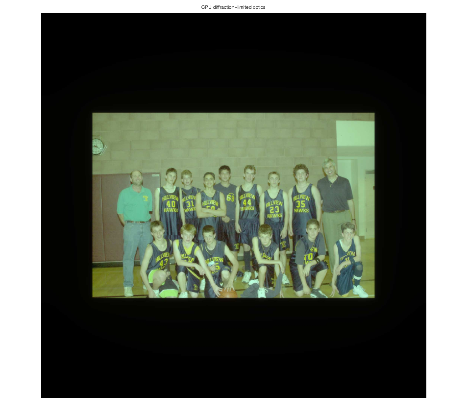
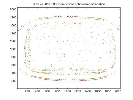
The diffraction-limited optics has good performance and excellent accuracy. Computing the diffraction-limited OTF on the GPU seems have a positive impact on accuracy along with increased performance.
The error contours for the basketball image are circular probably reflect the difference between the single-precision OTF calculation on the GPU and the double-precision computation on the GPU.
|
|
|
|
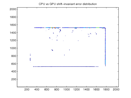
The performance improvement using the GPU is signficant; however, the PSNR is relatively low. As shown in figures 13, 15, and 17, most of the error is located on edges. GPU performance scales almost linearly with the number of GPU threads too. Using bilinearing interpolation during rotation on the GPU slightly increases PSNR while increasing run-time by about 20 percent over the point interpolation rotation method.
|
|
|
|
|
|
Using the GPU for optics computation is very beneficial. Computation run-time can be significantly reduced and still generate output with a reasonable peak signal to noise ratio. The performance improvement using the NVIDIA GeForce 9800 GX2 with ray trace optics is nearly two-orders of magnitude. Reducing the run-time from over a day to just under 18 minutes is very substantial. If the GPU computation results are unacceptable for the final simulation, it is still very useful in sweeping parameters during optics design. Using GPU acceleration, 80 lens could be simulated in the same amount of time as one on the CPU!
Diffraction-limited and shift-invariant optics provide a reasonable performance boost while mantaining high PSNR. The GPU code is not significantly optimized so there is definitely the potential for performance improvement. In particular, the compression operaton from double-precision floating point to the eight-bit char datatype is a good candiate for computation on the GPU.
The ray trace GPU optics code is highly optimized, it would be difficult to exact more performance on a current GPU. Future GPUs may offer more advanced features which could further increase performance. In particular, it may be possible to treat point spread functions as textures and rotate them in hardware. Rotation in hardware may not be possible but it is definitely worth further investigation.
If the rotation and interpolation kernels were modified by someone who has an indepth understanding of the algorithms used by MATLAB for imrotate and interp2, the PSNR could likely be increased without signficiantly impacting the run-time. If a GPU with double-precision support were used, some errors caused by casts between single-precision and double-precision variables would disappear.
GPU Code (includes modified ISET code)
1) Download the CUDA SDK and Driver from NVIDIA You'll also need a functional installation of MATLAB, ISET 3.0, and a C++ compiler. On Windows, you'll need a recent vintage of Visual Studio. On OS X, make sure the X Code developer tools are installed. Under Linux, make sure GCC is installed.
2) Make sure the CUDA libraries are in your path (under OS X and Linux add "/usr/local/cuda/lib" to LD_LIBRARY_PATH environment variable)
3) Make sure the CUDA compiler toolchain is in your path (under OS X and Linux add "/usr/local/cuda/bin" to PATH environment variable)
4) Compile NVIDIA CUDA demo code. The MATLAB code uses the libcutil library. This needs to get copied to compilation working directory. ( Copy libcutil.a from NVIDIA_CUDA_SDK/lib/ to where the optics code was uncompressed)
5) Run "nvcc -c bulk_rt.cu" to generate an object file (bulk_rt.o) for the GPU ray-trace code. For the shift-invariant code, run "nvcc -c filter.cu"
6) Build ray-trace MATLAB plugin by compiling "gpu_bulk_rt.cc" with MEX and linking with "bulk_rt.o". An example, "mex gpu_bulk_rt.cc bulk_rt.o libcutil.a -I/usr/local/cuda/include -L/usr/local/cuda/lib/ -lcudart -lcufft"
6) Build shift-invariant MATLAB plugin by compiling "gpu_filter.cc" with MEX and linking with "filter.o". An example, "mex gpu_filter.cc filter.o libcutil.a -I/usr/local/cuda/include -L/usr/local/cuda/lib/ -lcudart -lcufft"
7) Copy opticsOTF.m to ISET-3.0/opticalimage/optics and rtPSFApply.m to ISET-3.0/modules/raytrace
That should be it! If it doesn't work, feel free to email me
[1] Optical Research Associates. Code v.
[2] ImagEval Consulting. ISET digital camera simulator.
[3] NVIDIA Corporation. CUDA reference manual.
[4] NVIDIA Corporation. CUFFT library, 2007.
[5] NVIDIA Corporation. Tesla high performance computing, 2007.
[6] Zemax Development Corporation. Zemax.
[7] Matteo Frigo. A fast fourier transform compiler. In PLDI ’99: Proceedings of the ACM SIGPLAN 1999 conference on Programming language design and implementation, pages 169–180, New York, NY, USA, 1999. ACM.
[8] Alexander Huth. 2d CUDA-based bilinear interpolation, 2008.
[9] The MathWorks. Parallel computing toolbox 4.1.
[10] John Nickolls, Ian Buck, Michael Garland, and Kevin Skadron. Scalable parallel programming with cuda. In SIGGRAPH ’08: ACM SIGGRAPH 2008 classes, pages 1–14, New York, NY, USA, 2008. ACM.
[11] Muralidhara Subbarao. The optical transfer function of a diffraction-limited system for polychromatic illumination, 1988.