The color appearance of an object depends on the light that is reflected from the object and its neighbours. The spectrum of this reflected light depends not only on the surface reflectance of the object in question but also on the spectral composition of the illuminating light.
Human beings have some ability to compensate/disregard the illumination when judging object appearance. However the same doesn't hold true for various image capture devices where the same object will often look different under different illuminations.
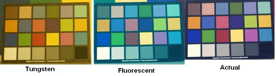
The image shown below(obtained from ImagEval website) of the Macbeth color checker under different illuminations provides an illustration of this fact.
The goal of color balancing algorithms is to carry out a global adjustment of the color intensities in an image so that the rendered image captures the true color characteristics of the object. Color balancing algorithms are used, not only in digital photography, but also in areas like machine vision, object recognition and other areas where the color of the object can be a key to obtaining a description of the object
Over the years a number of algorithms have been proposed to carry out the task of color balancing.
One of the oldest among these is the Gray World algorithm [1].
The Gray World algorithm is based on the assumption that the average reflectance of surfaces in the world is achromatic. Hence the algorithm applies a scaling factor to the R, G and B components of an image in such a way that they average out to a common gray value.
In recent years a number of other algorithms have been proposed for the task of color balancing. A few among them are the algorithms proposed by Brainard et al[2] and Sapiro[3] which are based on building model representations of the lights and surfaces in an image so as to estimate the scene illuminant.
In this report we provide an overview of the Color by Correlation [4] algorithm proposed by Finlayson and others.
The color by correlation algorithm is based on illuminant classification (estimation), i.e. choosing the illuminant of the scene from a set of possible representative illuminants. This set of illuminants is obtained by choosing a range of commonly occuring indoor and outdoor illuminations.
Also, the chromaticity space under consideration ( say (Cr,Cb) or (x,y) or any other similar chromaticity space ) is divided into a set of uniformly spaced regions. This is a reasonable operation because of the following reasons :
The color by correlation algorithm uses a matrix M that defines a probability for each chromaticity-illuminant pair as shown in the image below.
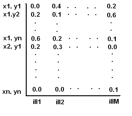
The column names - ill 1, ill 2 etc. represent the different illuminants in our representative set. The rows - (x1,y1) , (x1,y2) etc. represent each distinct region in our chromaticity space. As seen here, both chromaticity coordinates are divided into n distinct regions. Typical values of n are 16, 24 and 64.
Also, the chromaticity space is typically defined over the cube-root of our standard space ( i.e taking the coordinates as x^(1/3) and y^(1/3) ) as this leads to chromaticites which are uniformly distributed.
Each entry in the matrix M represents the logarithm of the probability that chromaticity i is observed under illuminant j. In other words each entry is equal to log( Pr( image chromaticity i | illuminant j ) ).
Details on how to construct the matrix M follow in the next section.
Assuming that we have the probability matrix M, color balancing for a image is carried out as follows :
We find the vector v = [ (x1,y1) (x1,y2) ... (xn,yn) ].
Each elemnt (xi,yj) of this vector is 1 if chromatcity level (xi,yj) occurs in the image and 0 otherwise.
Now we want to find the illuminant i such that Pr( illuminant i | Cim ), where Cim represents the set of chroma in the image, is maximised.
From Bayes rule, we know that
![]()
Assuming that the probability of any of the illuminants occuring is the same, the task of maximizing Pr( illuminant i | Cim ) is the same as finding the illuminant for which Pr( Cim | illuminant i) is the maximum.
The illuminant that maximizes this probability can thus be found by finding the product v * M. This product gives a value for each illuminant that is proportional to the Pr( Cim | illuminant i) . Finding the illuminant that has the maximum value in this vector gives us the illuminant that maximizes the probability of the image chromaticity.
The illuminant that leads to the highest probability of the chromaticity is taken to be the illuminant under which the scene was rendered. A simple linear transformation can then be used to transform the image color intensities into the color intensities that would be obtained if the image were rendered in, say, daylight.
To compute the probability matrix M, we take a collection of a large number of surfaces that are meant to be representative of object surfaces in the real world. In this case we used the set of 1995 surface reflectances available at the Simon Fraser University website.
For each of these surfaces we find the response of the surface under each of the illuminants in our set. The chromaticies thus obtained are used to produce a count for each chromaticity-illuminant pair which measures the number of times that chromaticity region was observed under that particular illuminant.
Normalizing the counts by the number of surfaces gives us Pr( image chromaticity i | illuminant j) and the logarithm of the same gives us the entries in the matrix M.
We choose the set of 18 illuminants available in ISET to be our set of representative illuminants.
We randomly chose surface patches and rendered them under different illuminants so as to create synthetic test images.
The images obtained were color balanced using the Gray World and Color by Correlation algorithms.
The color balanced images were then compared with the images of the same surface rendered under daylight. The CIE LAB metric was used for color comparison.
The figure below shows the average delta E obtained by averaging over 100 test synthetic images for each of the illuminants considered.
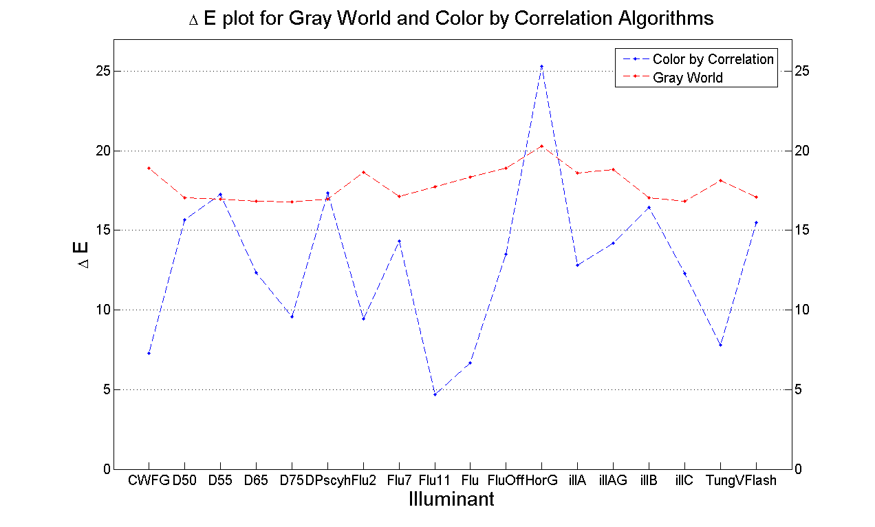
As we can see, the color by correlation algorithm performs better than the Gray world algorithm.
Also interesting to see is the percentage accuracy of the algorithm in terms of determining the correct illuminant. The figure below shows the percentage of times the algorithm correctly detected the illuminant in images that were synthesised under that illuminant.
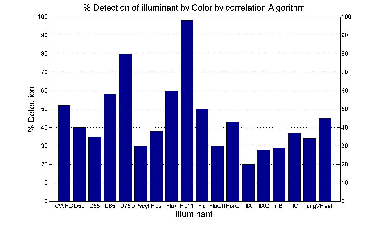
As we can see, the percentage detection of the illuminants is not very high. However, what seems to be more important is identifying the "type" of the illuminant.
For example, we noticed that many of the images renderend under D50, D55, D65 (daylights at different temperatures) were usually classified as being D75 lights. While this might have resulted in a less than optimal performance of the balancing algorithm, it doesn't seem to have affected the delta E scores adversly.
This seems to lead to the conclusion that we only need to maintain a carefully chosen set of representative illuminants.
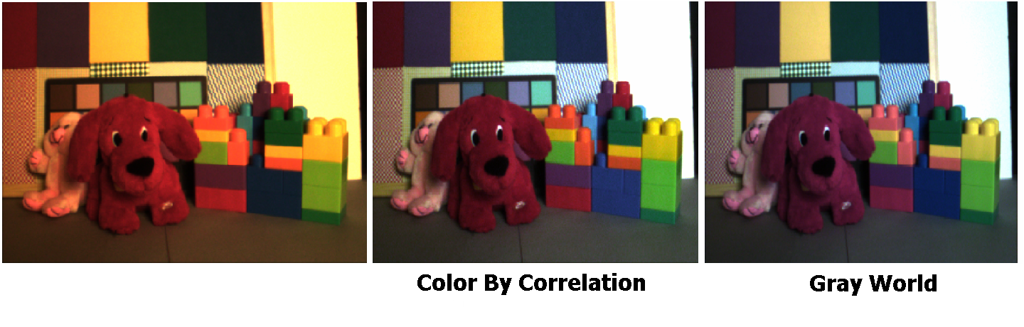
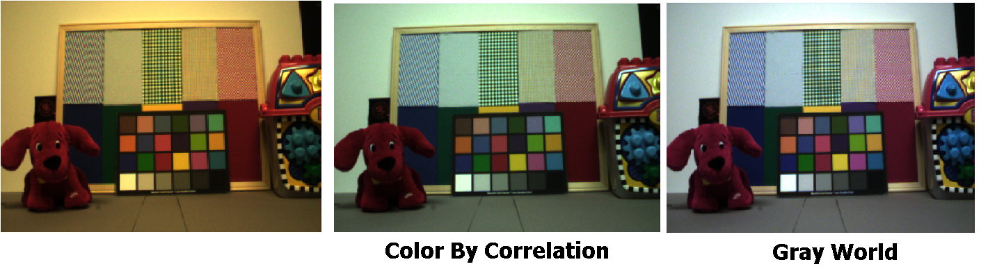
The following figures show the results that were obtained when the Gray World and Color by Correlation algorithms were applied to real world images.
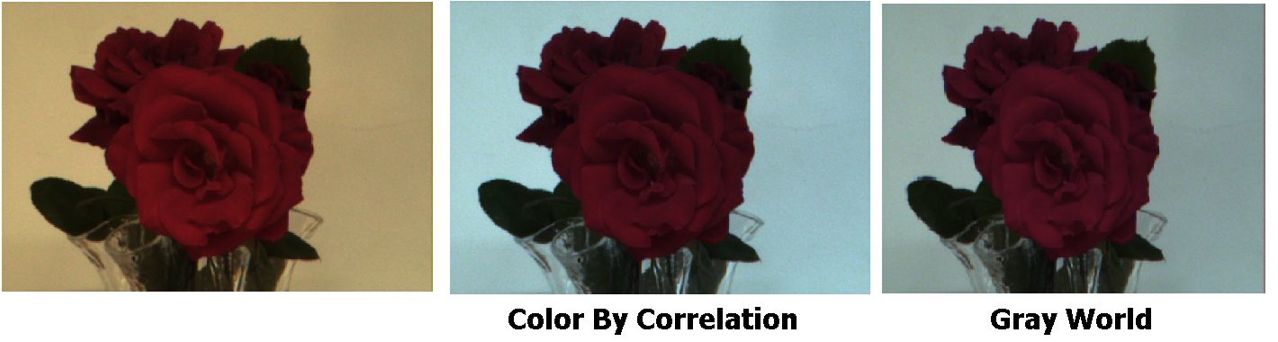
The color by correlation algorithm possesses some of the same disadvantages as the Gray World algorithm in terms of the algorithm not performing well when there aren't many surfaces in the image. An illustration of this is provided in the figure shown below
In conclusion, we see that the color by correlation algorithm seems to perform better than the gray world algorithm. However, it seems to be more important to estimate the class/kind of the illuminant rather than the illuminant itself. Also, we see that the algorithm is susceptible to some of the same problems as the gray world algorithm in terms of handling images that do not have many different surfaces in them.
[1] G. Buchsbaum. A spatial processor model for object colour perception. Journal of the Franklin Institute, 310:1-26, 1980.
[2] D. H. Brainard, W.T.Freeman. Bayesian color constancy. Journal of the Optical Society of America, A, 14(7):1393-1411, 1997.
[3] G. Sapiro. Color and illuminant voting. IEEE Transcations on Pattern Analysis and Machine Intelligence, 10:210-218, 1985.
[4] G.D. Finlayson, P.H.Hubel, S.Hordley. Color by Correlation, Proc. IS&T/SID Fifth Color Imaging Conference : Color Science, Systems and Application, pp 6-11, 2001.
Project presentation slides can be obtained here .
The program code is available here . (requires ISET toolbox)