Denoising
By Qun Feng Tan
Dept. of EE,
PSYCH 221 Project Winter 2008
I)
Introduction:
Usually, the acquisition of the image isn’t perfect and the result is a noisy image. Thus it would be practical to clean up the image first before running image-processing algorithms on it. Some image processing algorithms such as edge detection requires a relatively clean image to work well.
This project presents a study of various denoising algorithms, with comparisons of the pros and cons of the methods. We focus on several algorithms instead of just one, because there is no right algorithm to denoise a particular image. Denoising algorithms are usually selected based on some characteristics of the image known before hand.
There are many types of denoising techniques. We will select the most useful ones and show their application to simple cases.
II)
Methods
Denoising
Algorithms
Algorithm
1: Median Filters
The median filter is a non-linear technique for denoising. The fundamental
concept of the Median Filter is to select the most representative sample of a
window with odd dimensions. If the window is not of an odd dimension we
zero-pad it. We choose the sample which is most representative of that
particular window, i.e. the median of the pixel values, and discard the oldest
sample. A new sample is acquired, and the algorithm continues. To compensate
for the edge effects, we repeat the edge values. So lets say we have an array ![]() . We construct the following new array
. We construct the following new array
Y1 =
[X(1)*ones((window_size-1)/2,1);X;X(img_size)*ones((window_size-1)/2,1)];
before executing our median filter.
Here is a conceptual example of how the Median filter would work:
Suppose we have a linear array: [12 55 23 1 7] and we consider a sliding window-size of 3. The array that we start off with would be [12 12 55 23 1 7 7].
Output[1] = Median[12 12 55] = 12
Output[2] = Median[12 55 23] = 23
Output[3] = Median[55 23 1] = 23
Output[4] = Median[23 1 7] = 7
Output[5] = Median[1 7 7] = 7
Therefore the output image after passing through the median filter is [12 23 23 7 7]. Notice that the outlier 55 is removed.
At the end we would demonstrate the workability of the median filter on 1-bit images.
Algorithm
2: Hidden Markov Model (HMM)
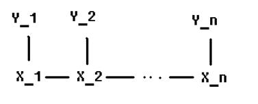
The concept of HMM can be applied to image denoising. In noisy image reconstruction, the estimator can be non-causal since the whole noisy image is already given. We can thus exploit the properties of HMM and derive algorithms where we can recursively apply to obtain the underlying clean image. The assumption here is that the states evolve according to a Markov Chain and the optimal Bayesian scheme can be implemented for prediction.
Here are the definition of some terms:
A
Markov Chain:
X – Y – Z if X is independent of Z given Y.
Thus ![]()
Hidden
Markov Process:
Suppose we have a Markov process ![]() , which we do not know. However, we have access to noisy
observations
, which we do not know. However, we have access to noisy
observations ![]() of
of ![]() . We can think of the
. We can think of the ![]() as the corrupted
image and the underlying
as the corrupted
image and the underlying ![]() as the clean
image.
as the clean
image.
If ![]() is formed by
passing
is formed by
passing ![]() through a
memoryless channel (the usual model assumption), then
through a
memoryless channel (the usual model assumption), then ![]() is known as the Hidden Markov Process and
is known as the Hidden Markov Process and ![]() is known as the
underlying State Process.
is known as the
underlying State Process.
We can represent our noise model as:
Derivation
of ![]() : Forward Recursive Algorithm
: Forward Recursive Algorithm
The Posterior Distribution of a random event is the conditional probability that is assigned when relevant observations are taken into account.
After computing the posterior distribution, we can use it to compute the optimum nonlinear estimator for the state estimation.
Define the following notational
simplification: ![]()

Next, note that we can also write

These 2 equations form the basis for the forward-recursion. The algorithm for the forward recursion can be formulated as follows:
Part 1: Forward recursive algorithm:
Goal: Determine ![]() for t = 1,…,n
for t = 1,…,n
1) Initialization:
i.
Some initial distribution ![]() à Setup to propagate the recursion.
à Setup to propagate the recursion.
ii.
Markov kernel: ![]()
iii.
Corruption channel (model by
which image gets corrupted): ![]()
iv.
Noisy observations: ![]()
2) Recursive step
For t = 1 to n step 1
 (Measurement
update)
(Measurement
update)
![]() (Time update)
(Time update)
End For-loop
Derivation of ![]() : Backward Recursive Algorithm
: Backward Recursive Algorithm
In image denoising, we already have the whole
dirty image available. Thus the whole time series is available to us. This
enables us to use a non-causal estimator to predict the underlying clean image.
That is, our goal is to find ![]() .
.
We have the following:
The above result allows us to present the Backward Recursive algorithm as follows:
Part 2: Backward recursive algorithm:
Goal: Determine ![]() for t = 1,…,n
for t = 1,…,n
1 - Initialization:
i.
From the Forward Recursive
Algorithm we have ![]() for t = 1,…,n à Setup to propagate the recursion.
for t = 1,…,n à Setup to propagate the recursion.
ii.
Markov kernel: ![]()
2 - Recursive step
For t = n-1 to 1 step – 1

End For-loop
At the end we would demonstrate the workability of the Forward/Backward Recursive Algorithm for 1-bit images.
Algorithm
3: Discrete Universal DEnoising Algorithm (DUDE)
This algorithm is a recent development (2005). The HMM method assumes an underlying Markov relationship in the state evolution. However, there are often times when the underlying state distribution is unknown, and so we cannot use the Bayesian Rule to compute the posterior distribution that easily. This is where the DUDE algorithm comes into play.
Fundamental concepts of the DUDE
algorithm:
Channel Model:
![]() , where A is the alphabet. Our objective here is to obtain a
set of values
, where A is the alphabet. Our objective here is to obtain a
set of values ![]() which will approximate
which will approximate ![]() as best as
possible according to some criterion (for example, minimizing some loss
function).
as best as
possible according to some criterion (for example, minimizing some loss
function).
Note that for the DUDE algorithm, we need
to have knowledge of several parameters beforehand. The channel statistics
should be known (![]() – the transition probability matrix). Also, a loss function
– the transition probability matrix). Also, a loss function ![]() should be specified.
For the purposes of this project, Hamming loss is assumed. (1 if
should be specified.
For the purposes of this project, Hamming loss is assumed. (1 if ![]() , 0 if
, 0 if ![]() ).
).
Step 1: First pass through the data set
– To compute count vectors
For a particular window of odd length, we have the following scenario:
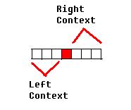
Let k be the context length. We see that ![]() where n is the
window length. The red pixel is the pixel we are concerned with.
where n is the
window length. The red pixel is the pixel we are concerned with.
In general, for ![]() , we define
, we define ![]() as the
M-dimension column vector whose
as the
M-dimension column vector whose ![]() component is equal to
component is equal to
![]()
The first pass of the DUDE involves
computing ![]() , where b and c represents the left- and right- context
respectively.
, where b and c represents the left- and right- context
respectively.
Step 2:
We correct each pixel according to this rule:
![]()
where ![]() and
and ![]() represents
component-wise multiplication.
represents
component-wise multiplication.
III)
Application of the Algorithms to cleaning images
As a proof of concept we demonstrate the power of the methods discussed above on 1-bit images, i.e. binary images.
To convert our normal image to bit images, we compare each pixel to the mean of all the pixels. We assign a 1 if that pixel value is greater than the mean, and a zero otherwise.
Suppose we have a binary image as follows. Each of the small boxes represent a pixel in the image.
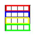
We vectorize the image above into a single row vector form – this models the time series that we would perform our algorithm on:
![]()
For the Forward/Backward Recursive
Algorithm, we have no way of determining ![]() since we do not
know the true distribution of the underlying. Thus, we can estimate the distributions
from the dirty image itself empirically.
since we do not
know the true distribution of the underlying. Thus, we can estimate the distributions
from the dirty image itself empirically.
After we have all our initializations, we can then proceed to execute the algorithms in MATLAB.
Corrupting the image
We corrupt the image pixel by pixel. We use MATLAB to generate a random number between 0 and 1. If the random number generated is less than p (the error rate of the image, which is the probability of corrupting the pixel), we corrupt the pixel by inverting the bit.
This corruption method is known as a Binary Symmetric Channel with error probability p:
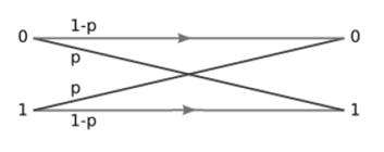
The transition matrix is given by ![]() .
.
For the DUDE algorithm, putting this into
our criterion ![]() and simplifying
we can get the following decision rule:
and simplifying
we can get the following decision rule:
IV)
Results
MATLAB results for an error rate of p =
0.25
Original Bit Image (of Albert Einstein):

Image after corruption with noise:
Images after denoising:
Part 1: For the Median Filter (Window length
= 9)
orig_error_rate =0.2491
post_error_rate =0.0986
Part 2: For the Forward/Backward
Recursive Algorithm (For 3 iterations)

orig_error_rate =0.2503
post_error_rate =0.0589
Part 3: For the DUDE Algorithm
orig_error_rate = 0.2508
post_error_rate = 0.0995
Performance of each algorithm for
different error rates
We run the algorithms for a different channel error rate and plot the performance level on a common axis so that we can make comparisons.
We can see from the graph that the Forward/Backward Recursive algorithm performs the best, The Median filter and the DUDE algorithm have approximately the same performance.
V)
Conclusion
The Median filter is conceptually simple to implement and runs fairly quickly. The error rate obtained is also reasonable given the method’s sophistication. This algorithm does make some assumption about the smoothness of the image.
Forward/Backward is very accurate as observed from the graph above.
However, one of the biggest disadvantages of the Forward/Backward Recursive Algorithm is the storage of data. For each step of the Forward/Backward Recursion we have to store all the posterior distributions. If the image is very big and the number of iterations involved is large, this can pose a problem.
DUDE algorithm is a new idea and is conceptually powerful. There are some adaptations of the DUDE out there that gives better performance rate for different situations (e.g. continuous-tone images). Even without making any real assumptions of the image, the algorithm still does very well. However, the DUDE algorithm takes an increasingly long time to run as window size and image size increases. This is because the different combinatorial possibilities of the contexts increases as well.
In conclusion, we see that different algorithms have different performance levels and characteristics. When denoising real-life images, we should pick the algorithm that best matches the characteristics of the image we are denoising.
VI)
References
1) T. Weissman, E. Ordentlich, G. Seroussi, S. Verdú, M. Weinberger. Universal Discrete Denoising: Known Channel
2) A. Buades, B. Coll, J. M. Morel. A Review of Image Denoising Algorithms, With a New One
3) L. R. Rabiner. A Tutorial on Hidden Markov Models and Selected Applications in Speech Recognition
VII)
MATLAB Code
MATLAB
CODE:
Link: denoising.zip
POWERPOINT
PRESENTATION: