"Measurements and correction of geometric distortion"

1. Introduction

   • 1.1 Image distortion

   • 1.2 Lens background

   • 1.3 Barrel and Pin-cushion distortion

   • 1.4 Camera Calibration

2. Geometric Distortion

• 2.1 Distortion Modeling Method

• 2.2 Polynomial and rational distortion functions

• 2.3 Simplified geometric distortion models

• 2.3.1 Model

• 2.3.2 Geometric undistortion

3. Results

• 3.1 Data

• 3.2 Measurements

4. Conclusion

5. References

6. Appendix

Report(.pdf)

Presentation(.ppt)

MATLAB code for GUI(.zip)

MATLAB code for distortion measurement (.m)

A perfect lens used in a camera would render straight lines as straight, no matter where they occur. But, consumer digital cameras are equipped with lenses that are not that good, and this results to changes in the geometry of the image. These effects are really disturbing in applications such as architectural shots, where the maintenance of straight lines is of critical importance. Geometric distortion is an error on an image, between the actual image coordinates and the ideal image coordinates. There are different types of geometric distortion are classified into the two following categories.

• internal distortion: resulting from the geometry of the lens
• external distortion: resulting from the attitude of the lens or the shape of the object

In the following figures (Figure 1.1 and 1.2) we present the different types of internal and external geometric distortion.

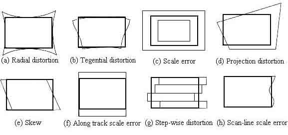
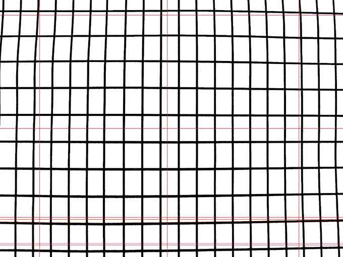
Figure 1.1: Internal Distortions

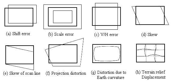
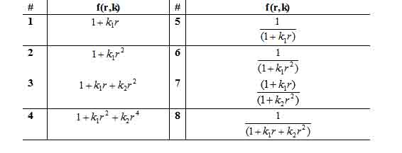
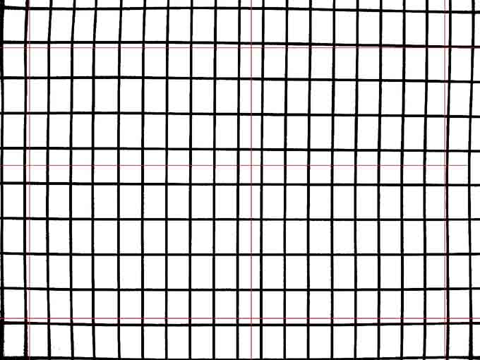
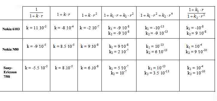
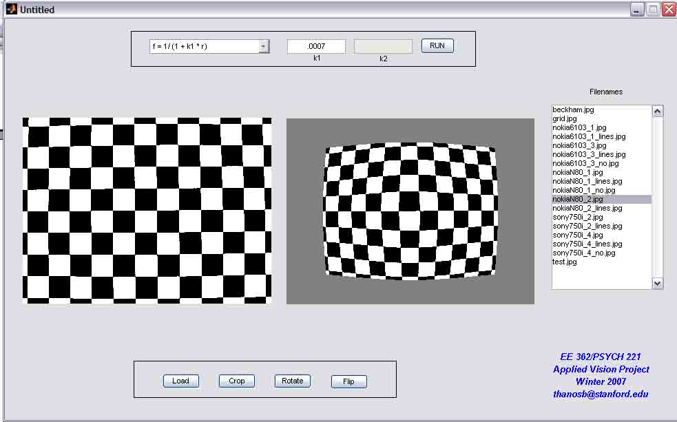
Figure 1.2 External Distortions

Among the above nonlinear distortions, the radial distortion which is along the radial direction from the center of distortion, is the most severe and the most common.

According to this type of geometric distortion, straight lines in the undistorted subject curve in the image taken by the camera. Straight lines that run through the image center (which in most of the cases is the same as the center of distortion) remain straight and a circle concentric with the image center remains a circle, although its radius is affected. Maybe the most typical cases of radial distortion are the barrel and the pin-cushion distortion, which we will analyze in a following section.

This paper reports on a method for modeling radial distortion. We are going to use six different models of distortion and measure the effect of each one of them, firstly on a picture of a grid and then on real grayscale images. We will see how the values distortion coefficients affect the distortion applied on the images and then we are going to use these models in order to calculate the distortion applied to images taken by the camera of a mobile phone.

A normal or standard lens is a lens that generates images that are generally held to have a "natural" perspective compared with lenses with longer or shorter focal lengths. In the case of this type of lenses, the exit angle of the image matches the entry angle, as shown in Figure 1.3.a.

A wide-angle lens is a lens whose focal length is substantially shorter than the focal length of a normal lens for the image size produced by the camera, whether this is dictated by the dimensions of the image frame at the film plane for film cameras or dimensions of the photosensor for digital cameras.

Finally, a telephoto lens is a specific construction of a long focal length photographic lens that places its optical center outside of its physical construction, such that the entire lens assembly is between the optical centre and the focal plane.

In the cases of wide-angle and telephoto lenses, when the lens has a field of view greater or smaller, respectively, the entry and exit angles are no longer the same. With a wide field of view the image has to be squeezed into a smaller space, as shown in Figure 1.3.b. The result is that scale and distance proportions between foreground and background are increased, therefore appear smaller as the distance between them and the camera is increased. On the other hand, when we use a lens with a narrower field of view, which is the case of telephoto lens, the image needs to be stretched to fit the space, as shown in Figure 1.3.c. The perspective is distorted in this case as well, but in the opposite way. This means that scale and distance proportions between foreground and background diminish so that objects that are far away from the camera appear larger than they are and sometimes equal to those who are closer to the camera. The result of this effect is that these two categories of objects appear to have no distance between them, something of course that is in contrast to the reality.

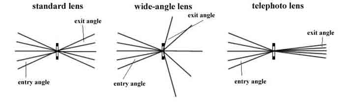
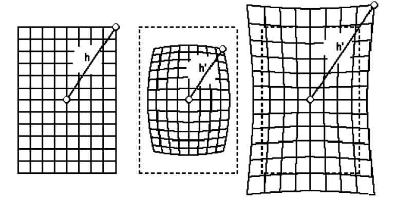
                                                (a)                                                     (b)                                                       (c)

Figure 1.3 Different types of lenses

The two typical lens distortion that occur are called barrel and pin-cushion distortion. They are named by the effect that they have upon an image, as shown in Figure 1.4. Barrel distortion is found in wide-angle views and it is the result of the squeeze that is applied in order to fit the image in a smaller space. On the other hand, pin-cushion is found in telephoto because of the stretching applied in the image in order to feet the space. The squeezing and the stretching of images vary radially due to the design of the lenses, making these distortions visually most prominent at the image corners and sides.

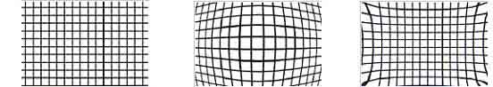
Figure 1.4 Original grid, barrel distortion and pin-cushion distortion

Corrective lens elements are used to reduce these faults as much as possible and some lenses exhibit much less distortion than others. The quality of a lens, and it's type, single focal length or zoom, usually determine how much distortion occurs. Lenses with single focal length, also called prime lenses, tend to produce less distortions because there are fewer elements and less need for optical compromise and it can be optimized for it's particular focal length, while a zoom involves many elements and some compromise, and the wider the focal range, the more compromise is involved. All lenses produce distortions, but they are hardly seen in the very best lenses, whilst in the cheaper types they may be quite prominent.

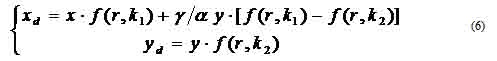
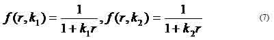
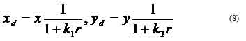
where

• r_u is the undistorted radius
• r_d is the distorted radius

Beside the two types of distortion mentioned above, there are also other more complicated types of distortion produced by lenses. A very common high order distortion pattern introduced by real-world lenses is the one that varies from barrel to pin-cushion across the field of the image. This distortion pattern is presented in Figure 1.5. The effect of such lens design is to have a maximum distortion mid-field, while the edges display little or virtually no distortion.

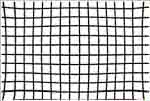
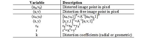
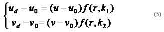
Figure 1.5 Higher order distortion

As we have mentioned previously, in practice, camera distortion could happen in a general geometrical manner that is not limited to the radial sense. Therefore, the commonly used radial distortion model for camera calibration is in fact an assumption or a restriction.

For many computer vision applications the camera is usually assumed to be fully calibrated beforehand. Camera calibration is the estimation of a set of parameters that describes the camera's imaging process. With this set of parameters, a perspective projection matrix can directly link a point in the 3-D world reference frame to its undistorted projection on the image plane. This is given by the following:

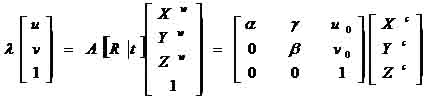
where (u, v) is the distortion-free image point on the image plane. The matrix A fully depends on the camera's five intrinsic parameters (α, γ, β, u₀, v₀) with (α, β) being two scalars in the two image axes, (u₀, v₀) the coordinates of the principal point, which generally fits in with the center of the image, and γ describing the skewness of the two image axes. [X^c, Y^c, Z^c]^T denotes a point in the camera frame that is related to the corresponding point [X^w, Y^w, Z^w]^T in the world reference frame by P^c = RP^w + t, with (R,t) being the rotation matrix and the translation vector.

In camera calibration, lens distortion is very important for accurate 3-D measurement [1]. The lens distortion introduces certain amount of nonlinear distortions, denoted by a function F in Figure 1.6, to the true image. The observed distorted image thus needs to go through the inverse function F^-1 to output the corrected image. That is, the goal of lens undistortion, or image correction, is to achieve an overall one-to-one mapping.

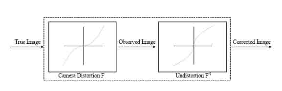
Figure 1.6 Distortion and Undistortion of image

Back on top

In this paper we present a simplified geometrical distortion modeling method by using two different radial distortion functions in the two image axes. A number of simplified geometric distortion models is presented, which are either simple polynomials or the rational functions of polynomials. This geometric modeling method is more appropriate for cameras whose distortion is not perfectly radially symmetric around the center of distortion.

As we have mentioned on the introduction of this paper, the radial distortion is the most severe part among the various nonlinear distortions [2],[3]. The removal of radial distortion is commonly performed by first applying a parametric radial distortion model, estimating the distortion coefficients, and then correcting the distortion. In most of the existing work, the radial distortion is governed by the following polynomial equation [4],[5],[6],[7]:

which is equivalent to

where k = [k1,k2,k3,…] is a vector of distortion coefficients.

For cameras whose distortion is not perfectly radially symmetric around the center of distortion, radial distortion modeling will not be accurate enough for applications such as precise visual metrology. In this case, a more general distortion model needs to be considered. In this paper, a simplified geometric distortion modeling method is presented, where two different functions in the form of a variety of polynomial and rational functions are used to model the distortions along the two image axes.

For real time image processing applications, the property of having analytical undistortion formulae is a desirable feature for both the radial and the geometric distortion models. Though there are ways to approximate the undistortion without numerical iterations, having analytical inverse formulae is advantageous by giving the exact inverse without introducing extra error sources. The simplified geometric distortion models that are presented in this project can achieve high calibration accuracy and better performance than their radial distortion modeling counterparts.

The variables that we are going to use in this project along with their description are presented in the following table, Table I.

Table I: List of variables

The commonly used polynomial radial distortion model is given in the form (1). As we previously mentioned, in this project, we are going to present both polynomial ad rational radial distortion functions [9],[10]. In the following table, Table II, we present the functions that we used in this project in order to distort or undistort an image.

Table II: Polynomial and rational distortion functions

As we can see from the Table II above, all these functions, except function #4, are special cases of the following radial distortion function having analytical inverse formulae:

The function #4 in Table II is in the form of (1) with two distortion coefficients, which is the most commonly used conventional radial distortion function in the polynomial approximation category.

For the functions mentioned in Table II, we must mention that they satisfy the following properties:

• The function is radially symmetric around the center of distortion and is expressed in terms of the radius r only
• The function is continuous and rd = 0 if and only if r = 0
• The approximation of xd is an odd function of x

The above three properties act as the criteria to be candidate for the radial distortion function. However, for the general geometric distortion functions, which are not necessarily the same along the two image axes, the first property does not need to be satisfied, though the functions need to be continuous such that there will be no distortion only on the center of distortion, which we assume that fits in with the center of the image in the case of this project.

A family of simplified geometric distortion models is proposed as

Where the distortion function f(r,k) in (3) can be chosen to be, though not restricted to, any of the functions in Table II. When k₁ = k₂ = k, the geometric distortion reduces to the radial distortion in equation (2). From (3), the relationship between (u_d,v_d) and (u,v) becomes

If we define

the relationship between (xd,yd) and (x,y) becomes

In this project we are going to use the pair (3),(4) of equations, but we are aware that similar results can be achieved using (5) and (6).

For the simplified distortion model (3), the property of having analytical undistortion formulae is not preserved for most of the functions in Table II as for the radial distortion. However, when using the function #5 and #6 in Table II, the geometric undistortion can be performed analytically. For example, when

from (3), we have

The geometric undistortion problem is to calculate (x,y) from (x_d,y_d) given the distortion coefficients (k₁,k₂) that are determined through the nonlinear optimization process. From equation (8), we have the following quadratic function for r

whose analytical solutions exist. The above quadratic form in r has two analytical solutions, where one solution can be discarded because it deviates from rd dramatically. After r is derived, (x,y) can be calculated from (x_d,y_d) uniquely. In this way the geometric undistortion using the function #5 in Table II can be achieved non-iteratively. For the function #6, a similar quadratic function in the form of

can be derived with

Back on top

3.1 Data

In this project we tried to measure the radial distortion that is applied to images taken by the cameras of mobile phones. In order to make these measurements, initially, we draw a grid, like the one shown in the following figure, Figure 3.1.

Figure 3.1: grid for the measurements of the distortion

Then, we used three different mobile phones to take pictures of this grid. The mobile phones that we used were the following:

• Nokia 6103
• Nokia N80
• Sony-Ericsson 750i

The following three figures, Figure 3.2, 3.3 and 3.4, show the photos taken by these three mobile phones

Figure 3.2: Photo taken by Nokia 6103

Figure 3.3: Photo taken by Nokia N80

Figure 3.4: Photo taken by Sony-Ericsson 750i

It is pretty obvious from the above pictures that barrel distortion is applied on the photo taken by the Nokia 6103 and pin-cushion distortion is applied to the other two photos taken by the other two mobile phones.

In the photos above, we have drawn some straight red lines in order to make easier to notice the distortion of the image.

3.2 Measurements

After getting these photos, from an approximate distance of 25-35 centimeters from the image of the grid, we measured the distortion of these three images in comparison to the initial image of the grid.

In order to make these measurements, we built a small script in MATLAB that compares the positions of certain pixels in the original image to the positions of the same pixels in the distorted image. In fact what we measured was the mean value of the movement of a point because of the distortion, i.e. the difference

where h and h' are shown in the following figure, Figure 3.5

Figure 3.5: the two different types of radial distortion

The measurements for the photos taken using the three different mobile phones mentioned above, are presented in the following table, Table III.

Table III: The measurements for the three mobile phones

The above results are not unexpected, since the Nokia 6103 is a three years old model and the other two are only one and a half years old. Therefore, we can see that there is an improvement on the quality of the photos that we can take using a mobile phone.

The m-file of the script that we used in order to make these measurements can be found in the Appendix of this project. There are comments in the MATLAB code in order to explain everything that is done by it and how these measurements come up.

Then we tried to correct the distortion that appeared in the photos taken by the three mobile phones. The way we did that was the following: firstly, we picked one of the distortion functions ( models ) mentioned above. Then we tried different values of the distortion coefficients for this distortion model and we applied it on the distorted image. In fact the model that we pick up must apply the inverse transformation of the one applied by the lens of the camera in order to get the undistorted image. In the following table, Table IV, we present the functions and the values that we used in order to get the undistorted images taken by the three different mobile phones.

Table IV: Models and coefficient values used to undistort the images

In what follows we present some pictures that show the steps of using different values of the distortion coefficient, while trying to get the undistorted image from the distorted one.

The values K₁, K₂, K₃, K₄, K₅ , in Figure 3.6, are increasing values of the distortion coefficient k that we use when we apply the distortion function

The fifth photo presents the undistorted image that we get for a value of k = 11×10-5 . The values of the coefficient that we used for the rest of the following images are:

K₁= 10^-6 , K₂ =5x10^-6, K₃ =2x10^-5, K₄ =7x10^-5, K₅=11x10^-5

The initial image is taken using the Nokia 6103 mobile phone. On the same way we can estimate the value(s) of the distortion coefficient(s) for the rest of the models and the other two mobile phones, or any other camera. When the error between the undistorted image that we get and the original image of the subject (not the one taken using the camera) is close to zero, then we have a good estimate of the distortion coefficient and generally of the transformation applied on the image by the lens.

Figure 3.6: Estimating the distortion coefficients

Back on top

As we saw in the previous parts of the project, radial distortion is the most severe and the most common type of distortion that is applied to the images taken by a camera. Especially, when we are talking about low cost lenses for cameras, like the ones we used in measurements taken for this project, this effect can be really disturbing and may give strange curves instead of straight lines. These changes may have the form of barrel distortion (as in the photo taken by the Nokia 6103) or pin-cushion distortion (as in the pictures taken by the other two phones that we used in our measurements).

In order to avoid this distortion, we can compute the distortion parameters and model the distortion of the image throw one of the models that we referred to in this project. Then, since we will know the values of the distortion parameter, we can apply the inverse transformation (model) to the image and get the undistorted image. After finding out the values of the distortion parameters of the lens of the camera, we just have to apply the same undistortion transformation (model) in the picture in order to get rid of the distortion applied on it.

In the measurements shown in this project we must take under consideration a small error, because of the error that comes up when we take the photos, since it is really difficult to hold the mobile phone in a steady position while taking a photo. Moreover, there may be some error because of small changes in the angle from which the photo is taken. This small change may be important when using cheap lenses like those used to build cell phone cameras.

In addition, we must mention that the models that we refer to in this project are working only for the radial distortion of the images. For all the other types of distortion, that were mentioned in the introduction of the project, we must use other types of models in order to correct the images. Maybe this could be a part of some future projects of this class, I order to have, finally, a compete group of reports about the phenomenon of distortion in images. On the same way, the GUI interface build for the radial types of distortion can be extended, so that it will be able to model other types of distortion that are not covered by this project.

Back on top

• "A family of simplified geometric distortion models for camera calibration", LiLi Ma, YangQuan Chen, Kevin L. Moore
• "Efficient Measurement and Correction techniques for lens distortion", Abhishek Das, Dinesh Patil.
• http://en.wikipedia.org/wiki/Wide-angle_lens
• http://www.dxo.com/intl/photo/dxo_optics_pro/overview/optics_geometry_corrections/distortion
• [1] Reimar K. Lenz and Roger Y. Tsai, "Techniques for calibration of the scale factor and image center for high accuracy 3-D machine vision metrology," IEEE Transactions on Pattern Analysis and Machine Intelligence, vol. 10, no. 5, pp. 713-720, Sep. 1988.
• [2] Frederic Devernay and Olivier Faugeras, "Straight lines have to be straight," Machine Vision and Applications, vol. 13, no.1, pp. 14-24, 2001.
• [3] Roger Y. Tsai, "A versatile camera calibration technique for high-accuracy 3D machine vision metrology using off-the-shelf TV cameras and lenses," IEEE Journal of Robotics and Automation, vol. 3, no. 4, pp. 323-344, Aug. 1987.
• [4] Chester C Slama, Ed., Manual of Photogrammetry, American Society of Photogrammetry, fourth edition, 1980.
• [5] Zhengyou Zhang, "Flexible camera calibration by viewing a plane from unknown orientation," IEEE International Conference on Computer Vision, pp. 666-673, Sep. 1999.
• [6] J. Heikkil and O. Silvn, "A four-step camera calibration procedure with implicit image correction," in IEEE Computer Society Conference on Computer Vision and Pattern Recognition, San Juan, Puerto Rico, 1997, pp. 1106-1112.
• [7] Janne Heikkila and Olli Silven, "Calibration procedure for short focal length off-the-shelf CCD cameras," in Proceedings of 13th International Conference on Pattern Recognition, Vienna, Austria, 1996, pp. 166-170.
• [9] Richard Hartley and Andrew Zisserman, Multiple View Geometry, Cambridge University Press, 2000.
• [10] Lili Ma, YangQuan Chen, and Kevin L. Moore, "Rational radial distortion models with analytical undistortion formulae,"Submitted for Journal Publication, http://arxiv.org/abs/cs.CV/0307047, 2003.

Back on top

In this part of the project we are going to give an overview of the GUI that we build in MATLAB. This GUI can be used in order to simulate the different types of distortion models that were presented in the previous pages and present the results of the application of these models in grayscale pictures. The pictures must be in the JPEG format (having a .jpg extension) and even if they are colored pictures, the distortion model is going to be applied only on the grayscale version of the image, and as a result the distortion image is not going to be a colored image.

Description

The GUI has the following form and can run by executing the command handler in the MATLAB command window. After the typing of the command handler and pressing enter we are going to get the following screen ( Figure A.1 ):

Figure A.1: The initial form of GUI

On the top of this window, we have a drop down list with the different functions (models) that we can use for the distortion of the image. Moreover, there is a drop down list where you can choose between having a correction in the distorted image or not. We will explain further what this means in the following paragraph. Then there are two forms where we give the values of the parameters of the distortion models that we will apply on the image.

In addition on the right side of this window there is a list of the .jpg files that are in the same folder with the MATLAB code and can be used for the distortion simulation. By clicking on the file name, and then on the button load we can see the image coming up on the left side of the screen, as it is shown in the following figure, Figure A.2:

Figure A.2: Loading a photo

Then, after choosing the function (model) that we want to use, choosing to correct the image or not, and giving the values of the model parameters, we click on the "Run" button and we get the distorted image, as shown in the following figure, Figure A.3:

Figure A.3: Applying distortion to an image

Then by using the "Crop" button and the mouse we can select a certain area of the image to apply the distortion model. Finally, by using the buttons "Rotate" and "Flip" we can flip or rotate the initial image before applying the distortion model on it.

Back on top