Non-Uniform Chromatic Aberration Compensation Using Colour Balancing Techniques

Problem Restated

The goal of this project is to investigate methods correcting non-uniform chromatic aberration caused by lens aberrations. These types of colour distortions can be dependent on either wavelength or spatial location within an image.

Chromatic Aberration

Figure 1: Chromatic Aberration - Left: Original Test Image, Right: Distorted Image

Chromatic aberrations manifest differently depending on whether they have a wavelength dependence or a spatial dependence.

Wavelength-dependent distortions cause colours to blur differently depending on wavelength, while spatially-dependent variations appear as an increasing blurring of colours as they move from the center of an image towards the periphery of the image.

Colour Balancing

We investigate how colour balancing techniques can be used to correct for these chromatic aberrations.

Figure 2: Image under Tungsten Lighting

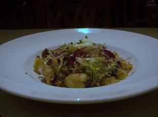
Figure 3: Image with Colour Balancing Applied

Traditional colour balancing techniques, typically attempting to compensate for differing illumination, are composed of two main steps:

1) Determining the type of illuminant found in an image, and

2) Adjusting the red, green, and blue (RGB) values of each pixel in a digital image to recover the original colour characteristics of the scene.

In typical implementations, RGB pixel values are transformed with a set of constants, resulting in a new colour balanced set of RGB values.

Colour Balancing Matrix

The set of constants used to transform a set of RGB pixel values is also known as a colour balancing matrix or kernel.

One way to think of colour balancing is taking the dot product of an RGB pixel value with a colour balancing matrix. The resulting vector is the colour balanced pixel value. Depending on the specific colour balancing algorithm, this operation is applied to every pixel within an image. The colour balancing may or may not be the same throughout the image. This also is dependent on the specific colour balancing algorithm.

Gray World

We investigate the use of a simple colour balancing algorithm called Gray World.

This particular algorithm makes no assumptions about the illiuminant, and attempts to compensate for different illuminants by augmenting an image so that each of the red, green, and blue colour channels of the image have identical means. With identical means for red, green, and blue, we say the image mean is gray.

When implementing Gray World, we adjust the means of the blue and red channels to match the green. Green is convenient because the human visual system is most sensitive to the colour green.

The colour balancing matrix is set to multiplicatively scale red pixel values to match the mean of all green pixels in the image, and similarly for blue pixel values. Green pixel

values are left alone. All non-diagonal entries of the colour balancing matrix are set to zero.

Compensating for Non-Uniform Chromatic Abberations

One goal of this project is to investigate strategies for using existing colour balancing algorithms to compensate for non-uniform chromatic aberrations, while simultaneously preventing the introduction of perceivable artifacts into the image.

The strategies presented are meant to be applicable for colour balancing algorithms other than Gray World, but Gray World is used as a representative of colour balancing algorithms that exist today.

Global Gray World

We begin by investigating what we call Global Gray World. A colour balancing kernel is generated from applying the Gray World algorithm to the entire image – that is, the mean red, green, and blue pixel values are calculated for the entire image, the values of which are used to create a single colour balancing kernel which is then applied to every pixel within the image.

Results

Figure 4: Left: Distorted Test Image, Right: Global Gray World Colour-Balanced Image

The results of Global Gray World are reasonable. At the center of the image, most of the original image’s colour characteristics are recovered. However, the non-uniform aberrations we are concerned about are still present at the extremes of the image – they are especially visible at the corners of the image. This is a result of the aberrations being proportional to distance from the center of the image, therefore the aberrations are worst at the corners.

Global vs Local Colour Balancing

The problem with Global Gray World is its dependence on a single colour balancing kernel to compensate for effects that vary throughout the image. A single colour balancing kernel is insufficient to handle aberrations at both the image center and periphery.

A possible solution is creating multiple colour balancing kernels, each using localized information – e.g., one kernel for the image center, another for the extreme edges of the image, and perhaps more in between. Each kernel would then be applied to the local area.

Localized Gray World

The Localized Gray World algorithm takes into account the fact that it is necessary to have multiple colour balancing kernels, each for varying spatial distances from the center of the image.

The image is split into several “zones”. Since we are concerned about spatially-dependent distortions, zones are comprised of all pixels that fall within a range of pixel distances away from the center of the image.

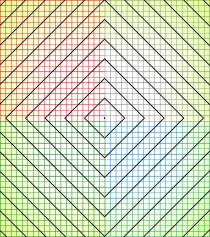
Figure 5: Distorted Image with Localized Gray World Zone Outline

Gray World is then applied to all pixels within each zone, and the resulting kernel from each zone is applied locally to all pixels within the zone.

Figure 6: Localized Gray World Model

Results

Figure 7: Left: Distorted Test Image, Right: Global Gray World Colour-Balanced Image

Localized Gray World performs well compensating for most aberrations at the center, as well as those at the image periphery. It is able to compensate for the perimeter chromatic aberrations that Global Gray World was unable to remove.

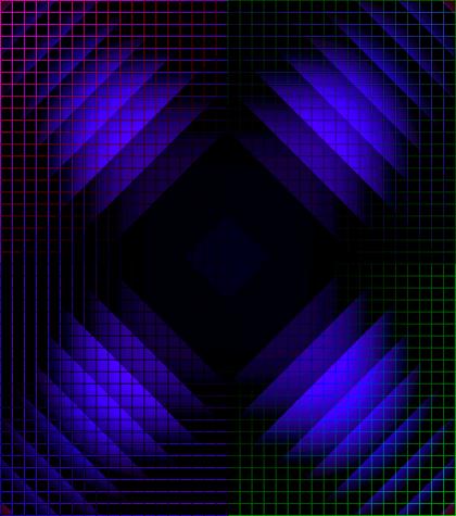
Figure 8: Difference between Original image and Localized Gray World Colour Balanced Image

However, since Localized Gray World uses separately calculated Gray World kernels for each zone, with potentially extreme differences between each zone kernel, artifacts result at the borders between adjacent zones.

The image shows the difference between the colour-balanced image and the original image, and shows the border artifacts.

Smoothing Kernels

One potential solution to eliminating border artifacts is the smoothing of kernel values with neighbouring pixels. It is possible to implement smoothing by building a mask of Localized Gray World kernels for the entire image, after which a smoothing kernel, such as a Gaussian, can be applied.

Results

Figure 10: Left: Localized Gray World Border Artifacts, Right: Localized Gray World With Smoothed Kernels and Reduced Border Artifacts

Figure 10: Difference Images with Original. Left: Localized Gray World Border Artifacts, Right: Localized Gray World With Smoothed Kernels and Reduced Border Artifacts

Smoothing can be an effective solution for eliminating border artifacts, but implementation can be memory intensive because of the need to keep multiple kernels in memory for blurring, and can be computationally intensive.

Reducing Zone Size

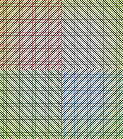
Figure 9: Localized Gray World Zone With Reduced Zone Size Outline

Another potential solution to the border artifact problem is the reduction of the local zone size.

As the scene changes radially, each zone is able to capture the subtle colour balancing changes necessary to make border artifacts less apparent.

However, there are several potential problems to this strategy. Since the Local Gray World algorithm uses the zone information to calculate the colour balancing kernel, there is much less information to calculate the matrix, and the calculated kernel may calculate a visually unappealing kernel, thereby creating an artifact that is as perceivable as the border artifacts when performing Localized Gray World with large zones. Essentially, each zone is a border artifact on its own.

This method may also be computationally intensive because each zone needs to calculate a separate kernel, and there are far more zones to work on, despite requiring less data per zone.

Results

Figure 10: Left: Localized Gray World Border Artifacts, Right: Localized Gray World With Reduced Zone Size and Reduced Border Artifacts

In a non-adversarial image, however, results are very reasonable, with minimal perceivable border artifacts.

Reducing zone sizes would be a good strategy for hard-coded. For example, a camera could hold multiple hard-coded kernels varying with distance from the center of the image, and use this strategy of having many kernels in succession be pieced together to compensate for non-uniform chromatic aberrations with minimal perceivable artifacts.

Localized Gray World with Polynomial Fit

While chromatic aberrations are visually unappealing, we do not want to introduce additional artifacts in the process of removing them.

Working with Localized Gray World, we know that working with large zones and having jumps in kernels can create border artifacts, and we want to reduce the perceptual effect of those artifacts. We know we are attempting to correct chromatic aberations that are continuously changing as they move away from the center of the image. Therefore, as a corollary, reducing border artifacts can be accomplished by having the colour balancing kernels change continuously as they move away from the center of the image.

It is possible to smooth out the response of Localized Gray World. The colour balancing kernels being calculated would continue to be calculated on a zone-by-zone basis, but instead of applying the kernel directly to the zone, it is possible to create a continuous polynomial function that reflects the changes in each zone’s colour balancing kernel, which results in a smoothing out of the transitions between the zones.

The problem with this solution is increased computational complexity. It would be necessary for online hardware to calculate a polynomial function using each zone’s kernel, requiring more complex and undesired higher order arithmetic functions.

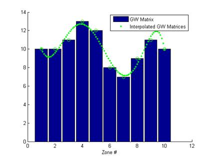
Figure 11: Localized Gray World Model with Polynomial Fit Interpolated Kernel Values

Localized Gray World with Linear Piece-Wise Interpolation

A compromise to make gains on computational complexity with some losses on smoothness of transition, while maintaining a continuous transition between zones is possible.

Instead of fitting a polynomial to the set of zone kernels, it is possible to perform a linear piece-wise interpolation between any two adjacent zones to calculate kernels for intermediate points in the image. This maintains a continuous change between zones, thereby minimizing perceivable border artifacts, while eliminating the need for calculating a polynomial fit for intermediate kernels.

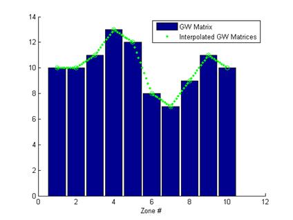
Figure 12: Localized Gray World Model with Linear Piece-Wise Interpolated Kernel Values

Results

Figure 13: Left: Distorted Test Image, Right: Localized Gray World with Linear Piece-Wise Interpolation Colour-Balanced Image

The Localized Gray World algorithm with Linear Piece-Wise Interpolation is able to correct most of the non-uniform chromatic aberrations found in distorted image and border artifacts are eliminated with continuous transitions between adjacent zones.

More Results

Additional test images show the results of using Localized Gray World with Linear Piece-Wise Interpolation.

In each image set, the top-left image shows the original, and the bottom-left distorted image exhibits wavelength-dependent and spatially-dependent chromatic aberration. The image on the right shows the results after applying Localized Gray World with Linear Piece-Wise Interpolation. Most aberrations found in the distorted image have been removed, and no border artifacts are visible.

While most of the images presented show that Localized Gray World with Linear Piece-Wise Interpolation is capable of removing spatially-dependent and wavelength-dependent chromatic aberrations at both the image center and periphery, the use of Gray World causes some colour changes in the image that are not present in the original. However, we are more concerned with the effectiveness of the overall colour balancing strategies presented, and in the case of Localized Gray World with Linear Piece-Wise Interpolation, for example, it is the concept of using linear piece-wise interpolation of colour balancing matrices to eliminate border artifacts that we are concerned about, not the explicit use of Gray World.

Animated Images

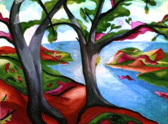
Figure 14: Top Left: Original Image, Bottom Left: Distorted Image, Right: Image corrected with Localized Gray World with Linear Piece-Wise Interpolation

Real World Images

Figure 15: : Top Left: Original Image, Bottom Left: Distorted Image, Right: Image corrected with Localized Gray World with Linear Piece-Wise Interpolation

Uniform Images

Figure 15: : Top Left: Original Image, Bottom Left: Distorted Image, Right: Image corrected with Localized Gray World with Linear Piece-Wise Interpolation