Light Falloff Analysis and Results

The images for the light falloff were analyzed using Matlab. The first step was to look at the global light falloff and determine if there were any effects from stray light or uneven illumination. If there was uneven illumination, then these images were rejected from the analysis. After the good images were identified, the normalized illumination level was calculated and a contour plot of the global light variation was made. The most interesting results were obtained by making a graph of the illumination level as a function of the radial distance from the center of the image.

In order to obtain the global variation in light level, the low frequency intensity variation needed to be separated from the background noise of the image pixels. This was done by applying an image filter in Matlab. With the high frequency components now suppressed, the contour command was used to create an image of the intensity contours of the image.

The source code for this analysis can be found here.

A. Filtering the usable images

The above method was applied to the images and then the image was either accepted or rejected depending on the intensity contours. Below is a sample of the images that were obtained from this processing.

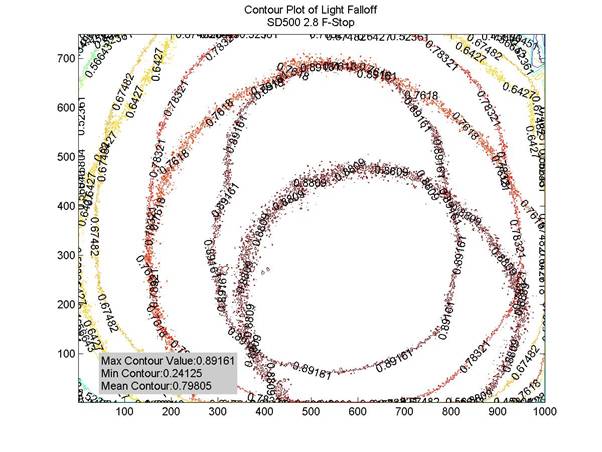
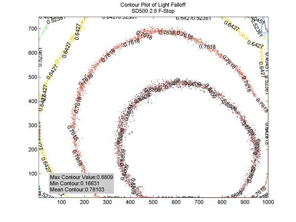
As an example, the first image in this series was rejected for the fact that there was an apparent effect from the stray light. The second image is a usable image. Note that the light falloff is not evenly distributed around the center of the image. This may signify non-uniform lighting, but this image warranted further investigation.

For the S50 camera, the results of the light falloff tests gave us mostly good images. As an example:

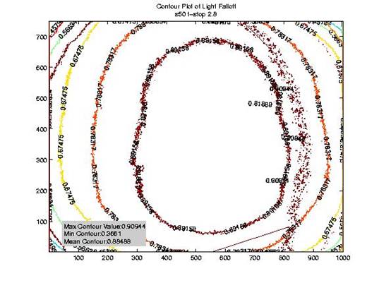
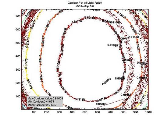
There is still some noise in the 5.6 f-stop image after filtering, but this is not too much of a concern for the comparison of light intensity versus radial distance. The trend will be somewhat noisy, but the trend will still be visible.

Follow this link for a full depository of test images.

B. Analyzing the light falloff

After the images were filtered, the image intensity as a function of the radial distance from center was analyzed for both cameras. A cut of the data was taken from the center of the image toward the corner of the image. The code for this analysis can be found here. In order to run this software, the clear all command needs to be suppressed so that for each time through, a new vector of intensity values is made. Then a command line needs to be run to plot all of the data on the same graph.

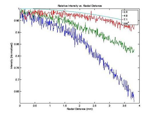
For each camera, the data for all f-stops was plotted on the same graph and compared to the cos⁴ function that is seen in natural vignetting. The results for the two cameras are presented below.

Relative intensity versus radial distance for SD500 camera:

Relative intensity versus radial distance for S50 camera:

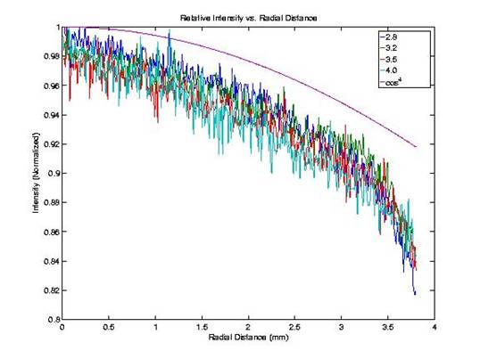
As can be seen from the graphs, the light falloff function for the SD500 camera is dependent on the f-stop. As the aperture size is decreased, the light falloff in the SD500 camera approaches the theoretical cos⁴ function. This suggests that the SD500 suffers from optical vignetting and the lens blocks some of the light when the aperture is wide open. For the S50, the intensity versus radial distance has the same curve regardless of the f-stop. This suggests that the S50 camera only suffers from light falloff due to natural effects. It would seem that the lens design, in terms of vignetting, is better in the S50 camera.

These differences may be due to different image processing performed on the two images. In the future, it may be interesting to compare the results from the raw, uncompressed output.

Back to Table of Contents.