The
Inkjet vs. Laser
A. Justin Sabet-Peyman

Abstract
The goal of my project is to compare inkjet printers and laser printers. In this write-up, I discuss how each of these technologies operate and also discuss some novel applications of printing technology. In addition, I do an experimental simulation that compares the performance of an inkjet printer to a laser printer. My simulation focuses on gauging the accuracy of basic color depiction and the efficacy of simple spatial frequency representation. The methods used in this project can be used as a foundation for a more thorough and comprehensive comparison of particular printer technologies in the future.
Table of Contents
Printer Technologies – How Laser Printers Work
Printer Technologies – How Inkjet Printers Work
Printer Technologies – Novel Applications of Inkjet Technology
I recently had a work experience at a Kleiner-Perkins backed
In 2001, the home printing industry in the
Questions like these have motivated me to focus my project
on understanding and comparing two of the most common printer technologies:
inkjet and laser. In 1998, an EE362
student, Baldemar Fuentes, did a cursory comparison between inkjet and laser
printers in which he briefly explained some of the operating principles and
compared magnified printouts of random images. In this project, I hope to more
thoroughly develop how inkjet and laser printers work, highlight areas of
current research, and lay the framework for a more comprehensive experimental
analysis of color and spatial frequency representation in the future.
Printer Technologies – How
Laser Printers Work
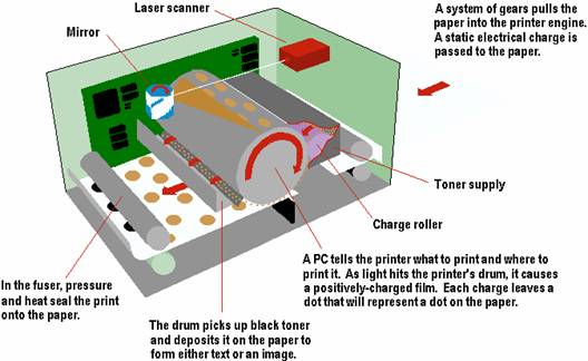
The laser printer was invented by a researcher at Xerox in 1971 and has been commercially available since 1976. Laser printers rely on static electricity to create images on paper. Static electricity is the electric charge that builds up on insulated materials. By manipulating this static electricity, laser printers are able to effectively bond toner to paper in patterns that correspond to the desired image. The three main parts of a laser printer are the drum, the laser, and the fuser.
The Drum
![]()
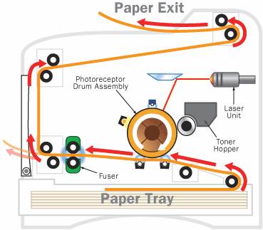
The drum is the main component in a laser printer and is oftentimes located near the center. It is usually made of a highly photoconductive material that can be charged or discharged by light. The drum interfaces directly with the paper and places the toner at the correct locations to produce the image.
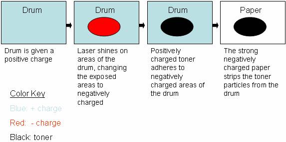
The way that the drum works is that it is given an initial charge to begin with. As the drum rotates in circles, the laser shines upon certain areas of the drum. The parts of the drum that get exposed to the laser experience a change in charge. For example, in certain laser printers, the drum is initially given strong positive electro-static charge and the laser causes exposed areas to change from a positive to a negative electro-static charge. In this way, the laser generates an electrostatic image on the drum.
Then, the printer exposes the rotating drum to positively charge toner particles. The toner particles are attracted to the negative areas of the drum that were exposed by the laser. As a result, the toner particles adhere to the areas of the paper corresponding to the electrostatic image. In this way, the toner is placed at the correct locations on the drum.
Then, the paper is given a strong negative charge (stronger than that of the drum) and is slid beneath the drum. Since the paper has a stronger negative charge than the drum, it takes the toner off of the drum so that the pattern from the drum is translated to the paper. Then, the paper goes through the fuser and the toner particles are fused into the paper.
The Laser
![]()
The laser is the part of the printer that actually draws the image onto the drum. As a result, it must be very accurate. The typical laser apparatus includes a laser, a movable mirror, and a lens to focus the light.
The laser itself does not move. It turns on and off according to the image that it is given. The mirror ends up directing the light such that the laser light shines upon the drum one horizontal strip at a time. The lenses focus the light further and give the laser apparatus the range it needs to traverse the width of the paper.
The Fuser
![]()
Laser printers do not use ink; instead, they use a substance called toner to image patterns on paper. Toner is an electrically charged powder that is made up of pigment and plastic. Since toner is solid, it does not spontaneously color the paper. Instead, toner must be physically fused into the paper with a fuser. The plastic in the toner enables it to be melted such that firmly bonds to the fibers within the paper.
As explained above, the charged toner particles adhere to the negatively charged areas of the drum that have been exposed by the laser. Then, the paper strips the toner off the drum and onto the paper. At that point, the toner is held to the paper by electrostatic forces. Then, the paper with the toner is passed through the fuser. The fuser heats the paper and the toner and causes the toner to melt such that it physically bonds to the fibers within the paper.
Printer Technologies – How
Inkjet Printers Work
HP Laboratories invented the first thermal inkjet technologies in 1979; however, it was not until the second half of the 1980’s that inkjet printers were introduced into the marketplace. Since then, they have grown in popularity and have stolen market share from laser printers.
Inkjet printers work in a much more intuitive way than laser printers. They essentially work by shooting ink onto paper. Both inkjet and laser printers are non-impact printers in the sense that they do not have mechanisms that physically touch paper in order to create images. However, unlike laser printers, inkjet printers use aqueous ink that spontaneously colors the paper (unlike toner from laser printers that has to be fused into the paper with a fuser).
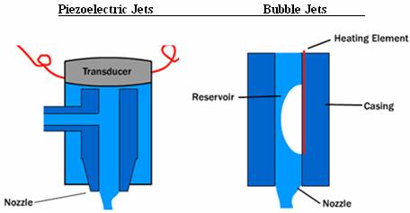
The core component of the inkjet printer is the print head that contains a series of nozzles that spray dots of ink onto paper. There are two main mechanisms that generate the spraying of ink from the nozzles. The first mechanism relies on a thermal bubble. In these systems, current flows through certain nozzles and heats up resistors near those nozzles. This heat vaporizes some the ink and generates a bubble that expands. As the bubble expands, ink is sprayed out of the nozzle. Then, the current decreases, and the bubble pops, sucking more ink from the cartridge to fill the empty space.
The other mechanism that inkjet printers rely on to spray ink from their nozzles involves piezoelectric materials. These materials change shape based on the electric field around them. A transducer is placed at the base (top) of the nozzle. An electrical stimulus excites the transducer so that it changes shape, causing ink to spray out of the nozzle. When the stimulus stops, ink from the reservoir flows back into the cartridge to fill the void.
Printing Technologies –
Novel Applications of Inkjet Technology
Inkjet printers are currently being used for much more than
simply putting ink onto paper. It has
been integrated into many fabrication methods for building three dimensional
parts. In particular, inkjet printers
are being used to print electrical and optical devices, especially where these
contain organic materials. For example,
Dr. Calvert at the
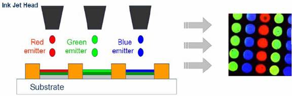
In addition to Organic Light-Emitting Diodes, researchers have also applied inkjet printing technology to create Sol-Gel materials, organic transistors, conducting polymers, structural polymers, ceramics, nanoparticles, metals, nucleic acids, and protein arrays.
Currently, many genomic researchers are applying inkjet printing to deposit DNA onto membranes. Reports in the scientific literature claim that DNA can be deposited onto membranes at 300 dpi using bubble-jet printers. Biologists have also used inkjet technology to print antigens onto polycarbonate materials for immunoassay. Engineers also use inkjet printers to fabricate small biosensors.
In addition, researchers have also used inkjet printing
technologies in various tissue engineering projects. Microfab, Inc. in
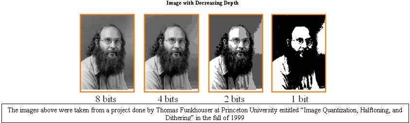
Both inkjet and laser printers are limited to just a few different colored inks, and yet they are able to produce many different shades of color. How are they able to do this? Many assume that printers work just like the television which has just three primaries but can create many different colors by changing the intensity of each of these primaries and adding them together. However, unlike televisions, most laser and inkjet printers are not able to change the intensities of their primaries. Most black and white laser printers, for example, only allow for a binary output of black or white, and most color printers contain only three or four colors of ink. How is it that a laser printer that only allows binary output of black or white for any given pixel location can produce the grayscale image on the left instead of the black and white image on the right?

Both inkjet and laser printers are able to achieve halftones through a process called dithering. Dithering takes advantage of the human visual system’s spatial resolution limitations to create the effect of multiple intensity levels. The human eye naturally blurs patterns with high resolutions according to the line spread function. Dithering takes advantage of this blurring to simulate the effect of observing different shades of gray.
The resolution of every static image depends on intensity resolution and spatial resolution. Intensity resolution is the “depth” of bits for representing intensities or colors within each pixel. Spatial resolution characterizes the number of or “width” x “height” of pixels within each image. For example, a binary output laser printer could have a spatial resolution of 6600x5100 with a depth of 1. One would expect, decreasing depth to look like the following:
However, dithering exploits blurring (or spatial integration) within the eye to render a large set of perceived intensities. In halftoning, printers use small patterns of dots to trick the human eye into seeing a particular intensity. In this way, a grayscale image with many shades can be successfully created. Each shade corresponds to a specific pattern of dots. The dots contain only one intensity; however, when viewed by the human eye from a distance, the pattern appears to have a color different than the color of the dot.
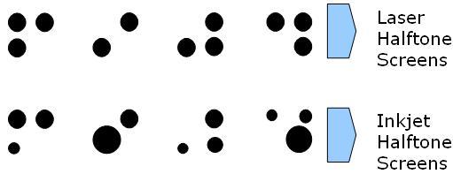
The pattern of dots used to represent a particular shade is referred to as a halftone screen. Most laser printers are only able to use dots of the same size because the dots are represented by toner particles. Since electrostatic charge is binary, toner particles are often the same size. (For example, if you wanted to use two different sizes of toner particles, you would need a ternary way of differentiating between the cases where you would want no toner particle, a small toner particle, or a larger toner particle.) However, inkjet printers do not face similar limitations; therefore, they can wield more flexibility because their halftone screens can contain dots of different sizes, yielding a larger array of possible shades.
Via these halftone screens, the printers simulate a broad range of different intensities, thus gaining intensity resolution (or “depth”) but losing spatial frequency. However, the human visual system is not sensitive to very high spatial frequencies. As a result, the loss in spatial frequency is not apparent to the viewer of the printed image while the gain in intensity resolution enhances the perceived image greatly.
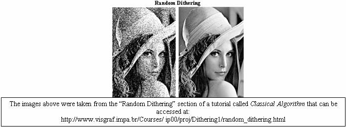
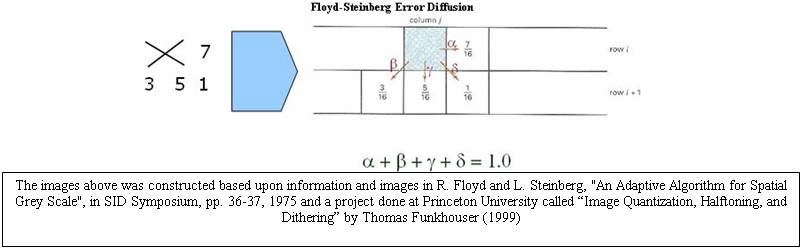
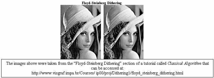
There are many different techniques used for dithering such as random dithering, ordered dithering, and Floyd-Steinberg dithering. In random dithering, you simply chose a random number between 1 and 256 for each pixel in the image. If the random value is greater than the grayscale pixel value, then that pixel becomes white and if not, that pixel becomes black. While this dithering process is simple, it creates lots of white noise.
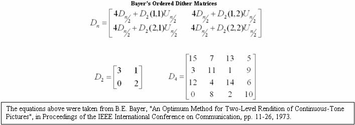
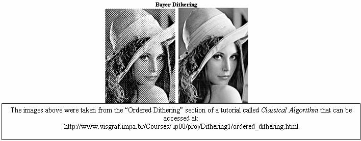
Ordered dithering techniques employ a matrix that contains a pattern of threshold values that can be compared to the pixel intensities to produce the discrete output of the halftoned image. B.E. Bayer showed in 1973 that for matrices of orders which are powers of two (of the type shown below), there is an optimal pattern of dispersed dots which results in the noise being as high-frequency as possible. Since the human visual system is less sensitive to high frequencies, the images look much cleaner.
Floyd-Steinberg dithering operates on the principle of error diffusion. It spreads the quantization error over neighboring pixels such that the error is dispersed to the pixels to the right and below as shown in the diagram.
Halftoning is also used to produce a large range of different colors. Again, halftone masks exploit the blurring of the human visual system to simulate different colors. The image below demonstrates how halftoning can create additional colors from just two colors. In this case, red and blue are used to create purple.
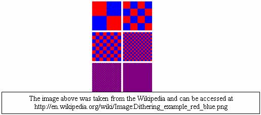
In most cases, color printers do not physically mix inks. Instead, they use halftone masks to cause viewers to perceive different colors. The mixing occurs within our eyes. For more information about color halftoning methods, consult the previous EE362 project entitled “Color Halftoning Techniques for Inkjet Printing” by Michael deLeon (2002).
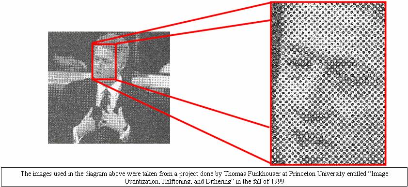
Overall, halftoning techniques are essential to both laser and inkjet printers. Any discussion of printer technologies would be significantly lacking without adequate credit given to the prominent role that halftoning plays in printing both grayscale and color images. As a final example of halftoning consider the following picture printout of Bill Clinton. After scanning in the image and zooming in, one could see that the shades of gray are achieved via the small halftone masks on the right.
Methods -
Color:
Summary: The goal of this experiment was to create colors with defined xy chromaticity values, to print out these colors with a chosen inkjet and a chosen laser printer, and to compare the xy chromaticity values for the printed sheets with the originals.
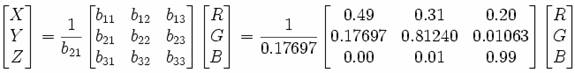
Use the following to go from RGB units to XYZ units:
Red:
See “Create_Red.m”
Matlab code
Output:
X_red =
2.7688
Y_red
= 1
Z_red =
0

Green:
See “Create_Green.m”
Matlab code
Output:
X_green = 1.7517
Y_green = 4.5906
Z_green = 0.0565

Blue:
See “Create_Blue.m”
Matlab file
Output:
X_blue = 1.1301
Y_blue = 0.0601
Z_blue = 5.5942

Gold
See“Create_Gold.m” Matlab file
Output:
X_gold = 4.6601
Y_gold = 4.9736
Z_gold = 2.1243

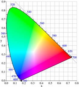
As we learned from our Color Matching Tutorial, the chromaticity of a color is determined by two variables x and y defined by the following:
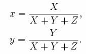
Therefore, we calculate the x and y values for each of the jpeg’s that we created:
Red:
X_red =
2.7688
Y_red =
1
Z_red =
0
>>
x_red = (X_red) / (X_red + Y_red + Z_red)
x_red =
0.7347
>>
y_red = (Y_red) / (X_red + Y_red + Z_red)
y_red = 0.2653
Green:
X_green = 1.7517
Y_green = 4.5906
Z_green = 0.0565
>> x_green = X_green / (X_green + Y_green + Z_green)
x_green = 0.2738
>> y_green = Y_green / (X_green + Y_green + Z_green)
y_green = 0.7174
Blue:
X_blue = 1.1301
Y_blue = 0.0601
Z_blue = 5.5942
>> x_blue = (X_blue) / (X_blue + Y_blue + Z_blue)
x_blue = 0.1666
>> y_blue = (Y_blue) / (X_blue + Y_blue + Z_blue)
y_blue = 0.0089
Gold:
X_gold = 4.6601
Y_gold = 4.9736
Z_gold = 2.1243
>> x_gold = X_gold / (X_gold + Y_gold + Z_gold)
x_gold = 0.3963
>> y_gold = Y_gold / (X_gold + Y_gold + Z_gold)
y_gold = 0.4230
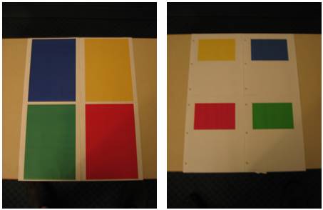
Next, I printed out the jpeg’s with a color inkjet printer and color laser printer to see how accurately they depict the target colors we have just created. The two printers that I used are the HP Color LaserJet 3700dn (left) and the HP Deskjet 3740 (right). (The reason the Inkjet printouts are smaller than the laser printouts is that I was trying to minimize cost by using less ink since, as we will discuss further in the conclusions portion, ink is expensive for inkjet printers):
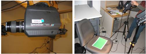
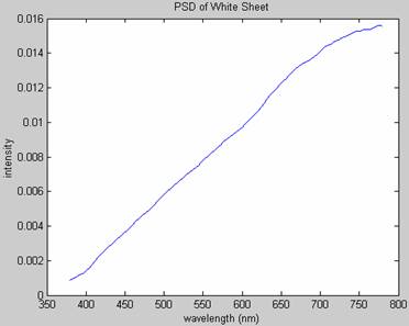
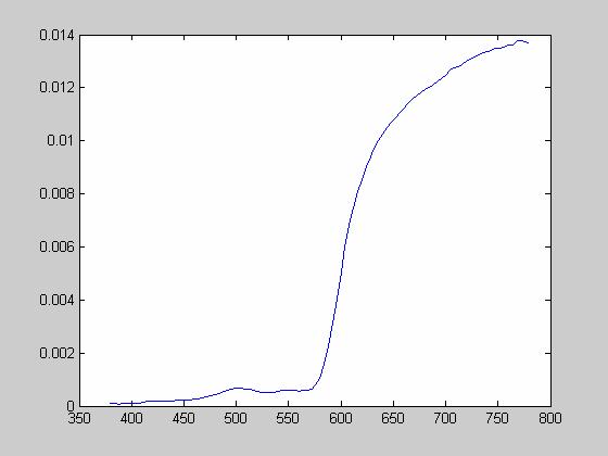
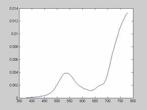
Now, we want to see how well these printouts depict the target colors of our jpeg’s. To do so, we have to use the Spectra Scan 650 to measure the power spectral density of each image:
In addition to reading the power spectral densities of the red, blue, green, and gold sheets from the laser and the inkjet printers, we also read the power from a blank white sheet as well. This reading gives us a frame of reference so that we could adjust all of our other readings so that they are independent of the ambient light that was in the lab when we measured the power spectral densities.
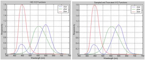
In order to account for the ambient light during the time of our measurements, I divided each power spectral density by the white sheet power spectral density to get the spectral reflectance of each surface. Then I calculated the XYZ of each image the same way that we did in our color matching tutorial by multiplying by the XYZ functions (however, I had to sample and truncate the functions to make sure that they matched up with our data from the Spectra Scan (see Matlab code). I plotted the sampled and truncated XYZ functions to make sure that they looked like the original XYZ functions from our tutorial:
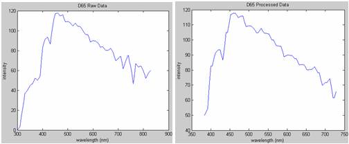
Next, I uploaded the power spectral density for d65 light. I used d65 light as my “standard” light source based on recommendations from the teaching team. Unfortunately, the raw data that I had was on a different wavelength scale than the spectral data from the Spectra Scan and the XYZ functions. As a result, I had to process the data to make sure that it would operate over the same wavelength vector. I checked plots (below) of my data afterward to make sure that the processing had preserved the signal’s integrity.
Once the power spectral density for D65 light had been
processed correctly, I multiplied each of the spectral reflectances for each
printout by the power spectral density of the D65 light above. This simulates
the situation when the printout is observed under “expected” or “standard”
light conditions. I used D65 light as my
standard because it is defined by the International Commission on Illumination
as a standard illuminating condition that corresponds roughly to midday sun in
Western /
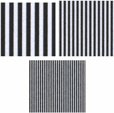
Summary: the goal of this experiment was to create images with 3 levels of spatial frequency in a vertical, horizontal, and rotated orientation, to print out these images with both the laser and inkjet printer, to scan the images back into the computer, and to compare the printouts. For this part of the project, I used inkjet and laser printers that both claimed to have 1200 x 1200 dpi. I used the HP Deskjet 3740 and the HP Laserjet 4100.
Vertical Spatial
Frequency
See
“Vertical_Spatial_Frequency.m” Matlab file
Output

Horizontal Spatial
Frequency
See
“Horizontal_Spatial_Frequency.m” Matlab file
Output

Diagonal Spatial Frequency:
See “Diagonal_Spatial_Frequency.m” Matlab file
Output
Next, I printed out the jpeg’s with an inkjet printer and a laser printer to see how accurately they depict the target colors we have just created. I used the same two printers as I used for the color experiment above, namely the HP Color LaserJet 3700dn (left) and the HP Deskjet 3740 (right). Both of these printers claim to print at 1200 x 1200 dpi. Then, I scanned the images in at 1200 x 1200 dpi using the Epson 3200 Perfection Scanner at the Meyer Multimedia Studio.
Using the Spectra Scan 650, I was able to measure power spectral densities for each of the printed sheets. To see the power spectral densities please consult the appendix. As mentioned above, I computed the XYZ values and the xy chromaticity values for each sheet and compared them with the original values. Here’s what I got:
(See
“Color_Analytics.m” Matlab file)
Here’s the spectrum of colors based on their xy chromaticity points. The “Error” value above corresponds to distance on this plot. For example, if the error is “.1” that means that the actual xy value and the measured xy value are .1 units apart on the plot below:
For each of the different colors, we determine which printer did a better job of producing the color such that it has an xy chromaticity value closer to the original xy chromaticity.
|
|
Inkjet Error |
Laser Error |
Δ Error |
Which is better? |
|
Green |
.218 |
.215 |
.003 |
Laser |
|
Gold |
.003 |
.017 |
-.014 |
Inkjet |
|
Blue |
.183 |
.157 |
.026 |
Laser |
|
Red |
.237 |
.202 |
.035 |
Laser |
|
Totals |
.641 |
.591 |
.05 |
Laser |
The chart above gives us an indication as to whether the inkjet or the laser printer produced more accurate colors for those tested.
Our second goal is to figure out whether or not there is a discernable difference between the colors generated by the inkjet and the laser printers. In order to do deduce this, we will have to calculate the CIELAB values for each of the printed sheets using the equations below:
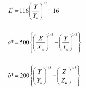
Note: we use the XYZ values of the white sheet reflectance as our white point values.
Then, in order to calculate the perceived difference between the colors generated by the laser printer and the colors generated by the inkjet printer, we calculate the delta_E value. The delta_E value gives us an indication of the perceived difference between the colors printed on the inkjet and the laser jet.
![]()
(See
“Color_Analytics.m” Matlab file)
|
Color |
Delta_E (Inkjet vs. Laser) |
|
Green |
10.3722 |
|
Gold |
6.2243 |
|
Blue |
7.6131 |
|
Red |
11.8276 |
Initially, my goal was to scan in the images from the various printers and compare them quantitatively. However, I encountered some significant problems when trying to do this. The first problem that I encountered had to do with the orientation of the images. No matter how hard I tried, it was difficult to make sure that the scanned images had perfectly balanced orientations. Even small imbalances of one to two degrees obscured my calculations. Likewise, I also encountered problems with size and position. Even though both my printouts contained 1200x1800 or 4x6in images, after scanning them in and cropping them, the sizes and positions were not consistent. As a result, my quantitative calculations did not produce clear results. Instead, I decided to rely on a qualitative assessment for spatial frequency.
Horizontal Spatial Frequency
Inkjet No Magnification (Highest Frequency)

The inkjet produces visible horizontal line artifacts for the highest frequency that are visible without any magnification.
Inkjet 10X Magnification
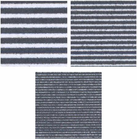
Laser 10X Magnification
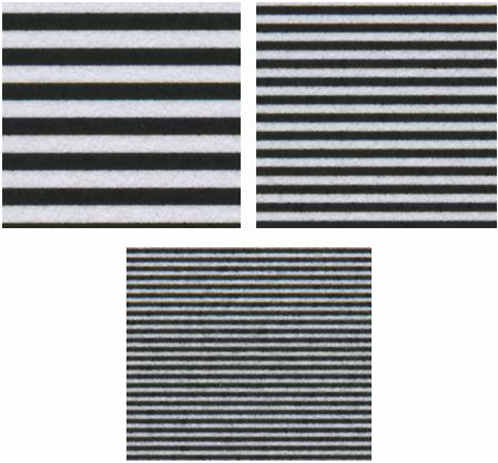
We notice that the laser printer produces a much crisper and cleaner printout at every one of the three frequencies. The Inkjet seems to smudge the ink, causing an erroneous image with more black than white (when there should be equal amounts of black and white).
Vertical Spatial Frequency
Inkjet 10X Magnification
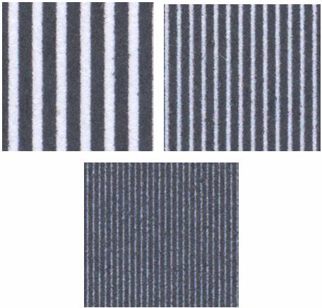
Laser 10X Magnification
Once again, the laser printer creates a much crisper and cleaner image. The inkjet printer smudges the ink so that there is erroneously more black than white (when there should be equal amounts of each color), especially in the higher frequencies. This smudging is more pronounced here in the vertical case than in the previous horizontal case.
Rotated Spatial Frequency
Inkjet 5X Magnification
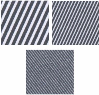
Laser 5X Magnification
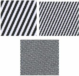
In this case, the inkjet printout looks a little bit smoother than the printout from the laser printer. Although we still see smudging in the inkjet printout, we notice that the quality of the rotated image is pretty similar to the quality of the horizontal and vertical images produced by the inkjet printer. However, the same cannot be said for the laser printer. Unlike the horizontal and vertical printouts, the rotated laser printout has jagged-edge artifacts that create a much noisier image at both low and high frequencies. Nonetheless, the laser artifacts seem to be repeated and ordered whereas inkjet artifacts tend to be more random as a result of the smudging..
The laser printers performed better than the inkjet printers in the simulations above; however, the simulations above were meant to serve as a foundation for a more comprehensive comparison that could be done in the future.
With regard to color, the laser printer did a more accurate job of generating printouts with colors more similar to the colors of the images. However, in the case of the gold image, the inkjet did a better job. The ΔE values between the green, blue, red, and gold laser printouts and inkjet printouts were all greater than 5, meaning that there was a perceivable difference, albeit a small one, between the laser printouts and the inkjet printouts. If I could do future tests (or if I were a future EE362 student), I would produce more color samples to confirm whether or not the laser printer exhibited better color resolution. Since there are an infinite number of possible colors, I would focus on the most commonly perceived colors.
With regard to spatial frequency, the laser printer generally produced crisper and more accurate images even though both printers claimed to operate at the same dpi. However, in the case of the rotated lines, the inkjet printer actually produced a smoother image. If I could do future tests (or if I were a future EE362 student), I would produce more diagonal and curved spatial frequencies to see if the inkjet continues to perform better. I would also produce colored spatial frequency samples to see whether or not color influences the resolution of the printouts.
The laser printers’ superior performance can in part be explained by the operating principles that we discussed earlier in the write-up. Laser printers use solid toner whereas inkjet printers use liquid ink. The ink from the inkjets visibly smudges, resulting in less crisp and blurrier images than those produced by the laser printer.
However, our discussion of laser and inkjet printers would be highly insufficient and irrelevant if we did not consider cost, which is oftentimes the most important factor driving adoption of printer technologies. The inkjet printer (DeskJet 3740) that we used in our experimental simulations costs $25 versus the laser printers (Color LaserJet 3700dn, and LaserJet 4100) that we used which cost $1200 and $500 respectively. Given that our inkjet printer is at least 25 times cheaper than each of the laser printers that we used, we note that it did a better job of representing color and spatial frequency relative to its purchase price. In addition, inkjet printers are also quieter than laser printers and do not require time to warm-up. This is why so many consumers have turned to inkjet printers and why they have stolen so much market share from laser printers.
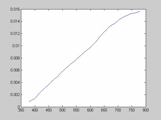
However, laser printers are more economical for high-volume purposes such as in offices. While laser printers cost more than inkjet printers, toner is much cheaper than the ink used in inkjets. As the chart below demonstrates, the total cost (including purchase price and toner/ink) for laser printers may become cheaper than an inkjet printer after a certain number of pages are printed. Other advantages of laser printers include speed and durability.
This
project was intended to establish methods for testing the color accuracy and
spatial frequency resolution of inkjet and laser printers. I would recommend that a future project do an
in-depth and comprehensive comparison between one particular laser printer and
one particular color printer, leveraging the operating principles and
experimental methods discussed in this write up. For color accuracy, I would suggest using a
much larger range of colors (ideally one that corresponded to the most
frequently observed colors). For spatial
frequency, I would suggest generating many more curved and diagonal images to
observe whether or not the inkjet does indeed perform better for certain types
of images. In addition, I would recommend pursuing interviews with printer
researchers and developers to discuss the reasons behind the observed
differences in performance.
Calvert, Paul. (Department of Materials Science and
Engineering at the
Sen, Surajit. “Nanoprinting with Nanoparticles: Concept of a Novel Inkjet Printer with Possible Applications in Invisible Tagging of Objects”, Journal of Dispersion Science and Technology. Vol. 25, No. 4, pp. 523-528, 2004.
Takada, Kazumasa et. al. “Metal Mask Fabrication with an Inkjet Printer for AWG Phase Trimming Using a Photosensitive Refractive Index Change”, IEEE Photonics Technology Letters, Vol. 17, No. 4, April 2005.
B.E. Bayer, "An Optimum Method for Two-Level Rendition of Continuous-Tone Pictures", in Proceedings of the IEEE International Conference on Communication, pp. 11-26, 1973.
R. Floyd and L. Steinberg, "An Adaptive Algorithm for Spatial Grey Scale", in SID Symposium, pp. 36-37, 1975.
Funkhouser, Thomas. “Image Quantization, Halftoning, and
Dithering”,
Classical Algorithm. Sections on “Ordered Dithering”, “Random Dithering”, and “Floyd-Steinberg Dithering”.
http://www.visgraf.impa.br/Courses/ip00/proj/Dithering1/floyd_steinberg_dithering.html
http://www.visgraf.impa.br/Courses/ip00/proj/Dithering1/ordered_dithering.html
http://www.visgraf.impa.br/Courses/ip00/proj/Dithering1/random_dithering.html
HP Invent, “Milestones in inkjet technology”,
http://www.hp.com/oeminkjet/learn/history/milestones.html.
“Color Halftoning Techniques for Inkjet Printing”, Michael deLeon, EE362 Final Project (2002)
“Laser Printing Devices”, Frederic Dalle, EE362 Final Project (1997)
EE362 “Tutorial
2: Color Matching”
EE362 “Tutorial
3: Color Metrics”
EE362 “Tutorial
4: JPEG”
EE362 Lecture “Color and Pattern”
EE362 Lecture “Light Measurement”
EE362 Lecture “Spatial Pattern Sensitivity”
Harris, Tom. “How Laser Printers Work”. HowStuffWorks. Main Computer Peripherals.
Tyson, Jeff. “How Inkjet Printers Work”. HowStuffWorks. Main Computer Peripherals.
http://www.bizstats.com
Wikipedia: http://en.wikipedia.org/wiki/Image:Dithering_example_red_blue.png
Color_Analytics.m
%Color_Analytics.m
%This
file performs all the color analytics for the inkjet and laser printouts.
% green laser print : spectral(:,1)
% yellow laser print : spectral(:,2)
% blue laser print : spectral(:,3)
% red laser print
: spectral(:,4)
% green inkjet print : spectral(:,5)
% yellow inkjet print : spectral(:,6)
% blue inkjet print : spectral(:,7)
% red inkjet print : spectral(:,8)
% light: spectral(:,9)
%load Justin.mat
%The
line above produces an error on some versions of Matlab. If so, manually import
the wavelength and spectral excel spreadsheets.
%Note that here, our
wavelength vector is [380:4:780]
wavelength = wavelength(:,1);
for ii =1:9
figure;
plot(wavelength,spectral(:,ii));
max(spectral(:,ii));
end
% To
get spectral reflectance of surfaces, we divide by the power spectral density
of the white sheet. This helps
% us achieve a calibrated
value for our other psd measurements that removes the effects of the particular
lighting
% that we were using at the
time of the measurement
light = spectral(:,9);
light = (light / max(light)) * max(spectral(:));
figure; plot(wavelength, light);
for ii = 1:9
reflectance(:,ii)
= spectral(:,ii) ./ light;
figure;
plot(wavelength,reflectance(:,ii));
end
%Now
we need to sample and truncate data65 such that it falls within 384:4:728;
%Once we do that, we will
multiple data65 by all the psd's and then we will compute the
%XYZ values of the new psd's
and the xy chromaticity points of those psd's. This is because
%the d65 gives us an
indication of how color appears in a normal ambient light which will serve
%as a good
basis to measure the color accuracy of the system.
load D65;
figure;
plot(wavelength,data);
title('D65 Raw Data')
xlabel('wavelength (nm)')
ylabel('intensity')
%Note that wavelength here is
[300:5:830]; we need to adjust data and wavelength such that they are on the
[384:4:728] scale.
%We
could do this by first expanding wavelength and data so that they are
[300:1:829] and then we truncate and we sample
%every
fourth.
%There
are 530 values from 300:1:829
%data65 = [1, 530];
%There
are 106 values from 300:5:829
k=1;
for
i = 1:106
data65(1,k) = data(i);
data65(1,k+1) = data(i);
data65(1,k+2) = data(i);
data65(1,k+3) = data(i);
data65(1,k+4) = data(i);
k = k+5;
end
%plot to see if the plot looks
approximately the same after the scale conversion
plot([300:1:829], data65)
%After
confirming that the plot does look the same, now we need to truncate the vector
%from [300:1:829] to [384:1:728];
note that 384 is the 85th value and 728 is the 429th value
%of [300:1:829]
data65_trun = data65(85:1:429);
%Now
we want to sample at every fourth value so that we are left with a vector that
traverses
%the data values from
wavelength = 384nm to wavelenth = 728nm by fours
data65_sampled = data65_trun(1:4:345);
%As a
test, we plot our truncated and sampled values.
figure;
plot(384:4:728, data65_sampled)
title('D65 Processed Data')
xlabel('wavelength (nm)')
ylabel('intensity')
%Now our d65_sampled vector
contains the power spectral density of d65 light at wavelengths that
%correspond
to our spectral data values. We multiply each spectral reflectance by the d65
light to
%simulate
the case where the prinouts are appearing in "midday sun" in Western/Northern
Europe.
for ii = 1:9
reflectance65(:,ii)
= data65_sampled' .* reflectance(2:88,ii);
figure;
plot([384:4:728],
reflectance65(:,ii));
end
%Note that here our wavelength
vector is [370:1:730]
load XYZ;
XYZ = data;
plot(wavelength, XYZ)
xlabel('Wavelength (nm)'), ylabel('Responsivity')
legend('xbar','ybar','zbar');
title('CIE XYZ Functions');
set(gca,'xlim',[350 750]), grid on
%We
plan to conform both the spectral data and the XYZ functions to the following
wavelength vector: [384:4:728]
X = XYZ(15:359,1)';
X_Sampled = X(1:4:345);
Y = XYZ(15:359,2)';
Y_Sampled = Y(1:4:345);
Z = XYZ(15:359,3)';
Z_Sampled = Z(1:4:345);
XYZ_Sampled = [X_Sampled'
Y_Sampled' Z_Sampled'];
figure;
plot([384:4:728], XYZ_Sampled)
xlabel('Wavelength (nm)'), ylabel('Responsivity')
legend('xbar','ybar','zbar');
title('Sampled and Truncated XYZ Functions');
set(gca,'xlim',[350 750]), grid on
%Here
we're trying to compute the xyz values before multiplying by the d65 light
for ii = 1:9
figure;
plot([384:4:728], reflectance65(:,ii));
XYZ_color(:,ii) =
XYZ_Sampled' * reflectance65(:,ii);
xy_chromaticity_color(1,ii) =
XYZ_color(1,ii) / ( XYZ_color(1,ii) + XYZ_color(2,ii) + XYZ_color(3,ii) );
xy_chromaticity_color(2,ii) = XYZ_color(2,ii)
/ ( XYZ_color(1,ii) + XYZ_color(2,ii) + XYZ_color(3,ii) );
end
xy_chromaticity_color
%Now
we want to calculate the CIELAB values from our XYZ values. In order to do so,
we use the XYZ values of the
%white sheet
reflectance as our XYZ white point values. 1 = a, 2 = b, 3 = L;
for ii = 1:9
CIELAB(1,ii) = 500 * ( ( XYZ_color(1,ii) /
XYZ_color(1,9) )^(1/3) - ( XYZ_color(2,ii)/XYZ_color(2,9) )^(1/3) );
CIELAB(2,ii) = 200 * ( ( XYZ_color(2,ii) /
XYZ_color(2,9) )^(1/3) - ( XYZ_color(3,ii)/XYZ_color(3,9) )^(1/3) );
CIELAB(3,ii) = 116 * (
XYZ_color(2,ii)/XYZ_color(2,9) )^(1/3) - 16;
end
CIELAB
%Calculate Green Delta E
between 1 and 5
Delta_E_Green
= ( ( CIELAB(1,1) - CIELAB(1,5) )^2 + ( CIELAB(2,1) - CIELAB(2,5) )^2 + (
CIELAB(3,1) - CIELAB(3,5) )^2 )^(1/2)
%Calculate Gold Delta E
between 1 and 5
Delta_E_Gold
= ( ( CIELAB(1,2) - CIELAB(1,6) )^2 + ( CIELAB(2,2) - CIELAB(2,6) )^2 + (
CIELAB(3,2) - CIELAB(3,6) )^2 )^(1/2)
%Calculate Blue Delta E
between 1 and 5
Delta_E_Blue
= ( ( CIELAB(1,3) - CIELAB(1,7) )^2 + ( CIELAB(2,3) - CIELAB(2,7) )^2 + (
CIELAB(3,3) - CIELAB(3,7) )^2 )^(1/2)
%Calculate Red Delta E between 1 and 5
Delta_E_Red=
( ( CIELAB(1,4) - CIELAB(1,8) )^2 + ( CIELAB(2,4) - CIELAB(2,8) )^2 + (
CIELAB(3,4) - CIELAB(3,8) )^2 )^(1/2)
Horizontal_Spatial_Frequency.m
height = 1200;
width = 1800;
im
= zeros(height,width,3);
strip = zeros(1,1200);
strip(1:4:400) = 1;
strip(2:4:400) = 1;
strip(401:8:800) = 1;
strip(402:8:800) = 1;
strip(403:8:800) = 1;
strip(404:8:800) = 1;
strip(801:16:1200) = 1;
strip(802:16:1200) = 1;
strip(803:16:1200) = 1;
strip(804:16:1200) = 1;
strip(805:16:1200) = 1;
strip(806:16:1200) = 1;
strip(807:16:1200) = 1;
strip(808:16:1200) = 1;
strip = strip'
im(:,:,1)
= repmat(strip,1,1800);
im(:,:,2) = im(:,:,1);
im(:,:,3) = im(:,:,1);
image(im);
imshow(im)
imwrite(im,'horizontal_spatial_frequency.jpg','jpg');
Vertical_Spatial_Frequency.m
height = 1200;
width = 1800;
im
= zeros(height,width,3);
strip = zeros(1,1800);
strip(1:4:600) = 1;
strip(2:4:600) = 1;
strip(601:8:1200) = 1;
strip(602:8:1200) = 1;
strip(603:8:1200) = 1;
strip(604:8:1200) = 1;
strip(1201:16:1800) = 1;
strip(1202:16:1800) = 1;
strip(1203:16:1800) = 1;
strip(1204:16:1800) = 1;
strip(1205:16:1800) = 1;
strip(1206:16:1800) = 1;
strip(1207:16:1800) = 1;
strip(1208:16:1800) = 1;
im(:,:,1)
= repmat(strip,1200,1);
im(:,:,2) = im(:,:,1);
im(:,:,3) = im(:,:,1);
image(im);
imshow(im)
imwrite(im,'vertical_spatial_frequency.jpg','jpg');
Rotated_Spatial_Frequency.m
height = 1200;
width = 1800;
im = zeros(height,width,3);
strip = zeros(1,1200);
strip(1:4:400) = 1;
strip(2:4:400) = 1;
strip(401:8:800) = 1;
strip(402:8:800) = 1;
strip(403:8:800) = 1;
strip(404:8:800) = 1;
strip(801:16:1200) = 1;
strip(802:16:1200) = 1;
strip(803:16:1200) = 1;
strip(804:16:1200) = 1;
strip(805:16:1200) = 1;
strip(806:16:1200) = 1;
strip(807:16:1200) = 1;
strip(808:16:1200) = 1;
strip = strip';
im(:,:,1) = repmat(strip,1,1800);
im(:,:,2)
= im(:,:,1);
im(:,:,3)
= im(:,:,1);
image(im);
imr = imrotate(im,5, 'crop');
imshow(imr)
imwrite(im,'rotated_spatial_frequency.jpg','jpg');
Create_Red.m
red
= [1, 0, 0];
vert
= 1200;
hori
= 1800;
temp = zeros(vert,hori,3);
temp(:,:,1) = red(1);
image(temp);
pause(1);
imwrite(temp,'red.jpg','jpg');
XYZ_red
= 1/.17697 *
[.49, .31, .20; .17697, .81240, .01063; .00, .01, .99] * red';
X_red = XYZ_red(1,1)
Y_red = XYZ_red(2,1)
Z_red
= XYZ_red(3,1)
Create_Blue.m
blue
= [0, 0, 1]
vert
= 1200;
hori
= 1800;
temp = zeros(vert,hori,3);
temp(:,:,3) = blue(3);
image(temp);
pause(1);
imwrite(temp,'blue.jpg','jpg');
XYZ_blue
= 1/.17697 *
[.49, .31, .20; .17697, .81240, .01063; .00, .01, .99] * blue'
X_blue
= XYZ_blue(1,1)
Y_blue
= XYZ_blue(2,1)
Z_blue
= XYZ_blue(3,1)
Create_Green.m
green = [0, 1, 0];
vert
= 1200;
hori
= 1800;
temp = zeros(vert,hori,3);
temp(:,:,2) = green(2);
image(temp);
pause(1);
imwrite(temp,'green.jpg','jpg');
XYZ_green
= 1/.17697 *
[.49, .31, .20; .17697, .81240, .01063; .00, .01, .99] * green';
X_green
= XYZ_green(1,1)
Y_green
= XYZ_green(2,1)
Z_green
= XYZ_green(3,1)
Create_Gold.m
gold
= [0.985 0.864 0.371];
vert
= 1200;
hori
= 1800;
temp = zeros(vert,hori,3);
temp(:,:,1) = gold(1);
temp(:,:,2) = gold(2);
temp(:,:,3) = gold(3);
image(temp);
pause(1);
imwrite(temp,'gold.jpg','jpg');
XYZ_gold
= 1/.17697 *
[.49, .31, .20; .17697, .81240, .01063; .00, .01, .99] * gold';
X_gold
= XYZ_gold(1,1)
Y_gold
= XYZ_gold(2,1)
Z_gold
= XYZ_gold(3,1)
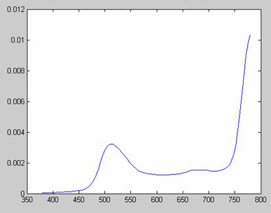
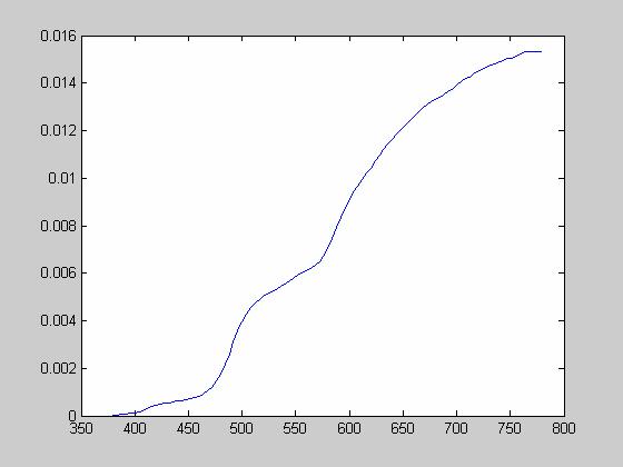
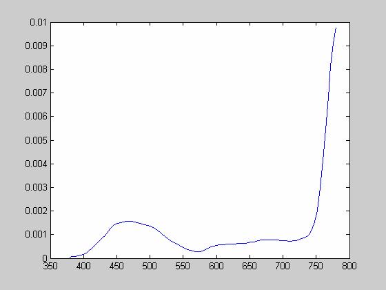
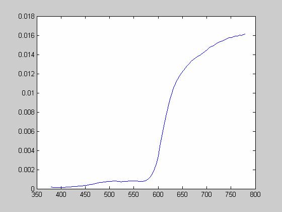
Appendix – Power Spectral
Densities from Spectra Scan 650
Green Laser:
Gold Laser:
Blue Laser:
Red Laser:
Green Inkjet:
Gold Inkjet:
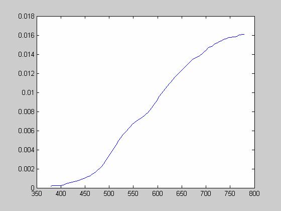
Blue Inkjet:
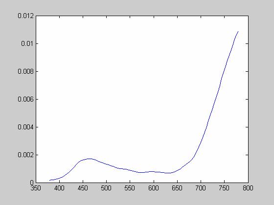
Red Inkjet:
White Sheet: