Formatting the bits of the watermark before embedding
Spread-Spectrum Technique
The spread-spectrum[14] techniques for watermark are very popular nowadays; the reasons will be
clear in the following paras.
The idea in SS is that the message used to watermark itself can be thought of a narrowband signal
compared to the cover image which is the wideband signal. Further, high frequencies are
not robust . The trick is to spread the watermark bits over the low frequency channels.
Kerckhoff's principle[16] states that we should try to hide the message or watermark in the
perceptually significant areas of the image. This is because if there is damage to the
watermark then the image is significantly altered enough to be useless anyways.
An important paper in the literature of Spread Spectrum and Watermarking is the paper by Cox et al[15].
It uses the above principle to accomplish watermarking using SS via the following algo:
The DCT of the image is first obtained.
Take the top n DCT coefficients where n is the length of the watermark
Spread the watermark over them with an invertible function
(the paper recommends [ v(i) = v(i)*(1+alpha*x(i)) ])
where alpha is the scaling coefficient
The key here is to note that each perturbation of the DCT coefficient is due
to x(i) and x(i) itself is chosen independently from a ~N(0,1) distribution
The inverse DCT is then taken and the image is ready to be sent
On the receiver side, we can extract X* (the process is detailed below). X* is nothing
but the values of X changed
The similarity of X and X*, which serves as a watermark detector, is then calculated using
sim(X,X*) = X*.X / sqrt(X*.X*)
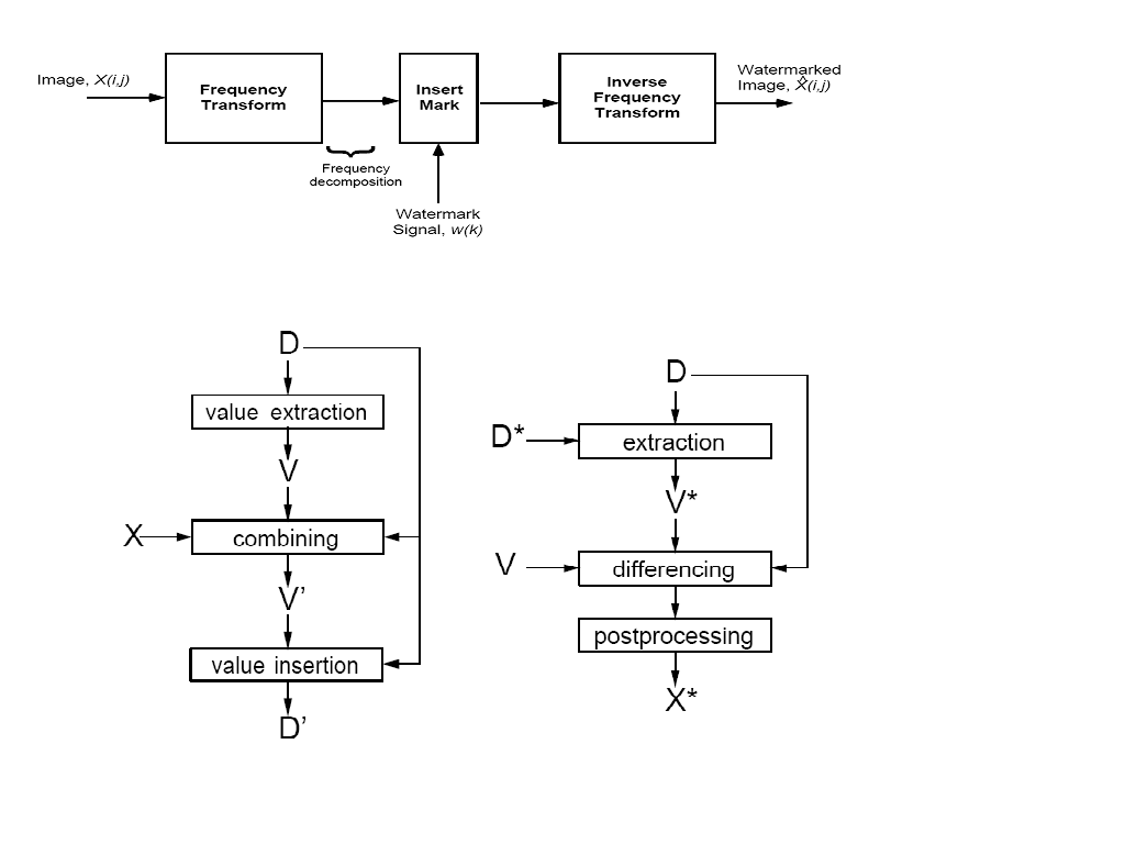
The overall process is further clarified by these images[15] showing the overall process
of encoding and decoding the watermark.
Implementation
I used the paper[15] by Cox et al. referred above as my base point and implemented the
following schemes:
Comparison with Random Watermarks
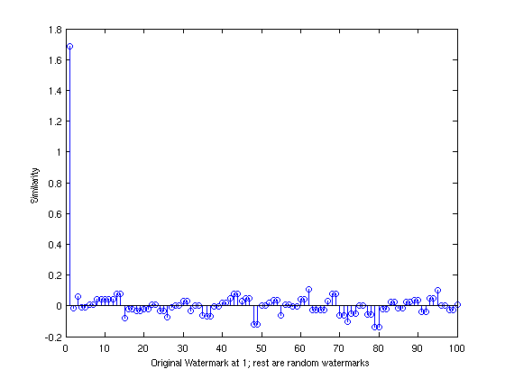
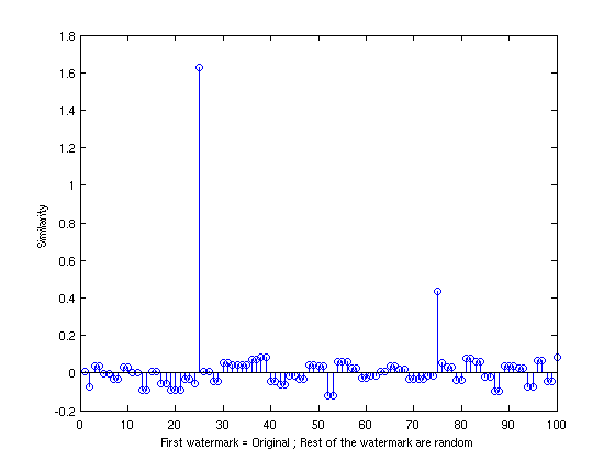
On the sending side, the standard Lena picture was taken and a watermark of 1000 bits was
applied to it using aforementioned algorithm. The receiving side used the similarity as a watermark detector
and plotted the similarity value against the Lena picture and 99 other randomly generated watermarks.
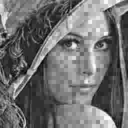
Original source image
One can see clearly that the similarity is very high when the real watermark is used. The random
watermarks pale in the similarity values. This is clearly because with random watermarks we
are essentially trying to find the similarity between two random normal distribtions which
will rightfully be very low.
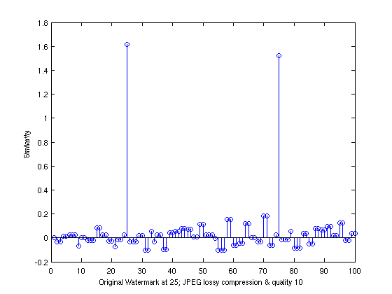
Comparison with JPEG lossy compressed/poor quality image transformation
The next test was with the watermarked image being JPEG lossy compressed with low quality (10%)
and then being decoded on the receiving end. Even with this the similarity value for the original
watermark is way higher than the random watermarks (though its obviously lower than the similarity value
of the original with itself)
JPEG lossy compressed Quality 10% image
Comparison with scaling and JPEG compression (decent quality)
The final test I did was to scale the image to 25% of its size in height and width
and use JPEG lossy compression with decent quality (75) and see how the watermark
detector performed using similarity value performed. The result was good though
obviously less emphatic than the previous cases but given the amount of transformation
to the image this method proved surprisingly effective.
Scaled Image after embedding watermark
Overall this Spread Spectrum method proved to be very effective in the tests I ran.