

Gregory Ng (gregng at stanford)
Stanford University
March 2005
In this project, I intend to characterize the noise present in output images from the Canon Powershot S1 IS. First, I will isolate the noise into a visually apparent form. Then, I will produce and analyze the statistics of the noise. Third, I will infer the sources of the noise. Finally, I will present several relatively simple methods for minimizing or removing the noise.
Noise can be classified into two forms: fixed-pattern noise and time-varying noise. Fixed-pattern noise generally has the same spatial arrangement and statistics from image sample to sample. Dark signal nonuniformity and photoresponse nonuniformity (PRNU) fall under this category. This type of noise is relatively easy to filter out, as you can find the mean value of the noise, and subtract this mean from your sample image.
The more interesting type of noise is time-varying noise. This noise varies spatially from sample to sample. Noise due to dark current, shot noise, and electrical system noise each fall under this category. This type of noise requires more advanced processing, described below.
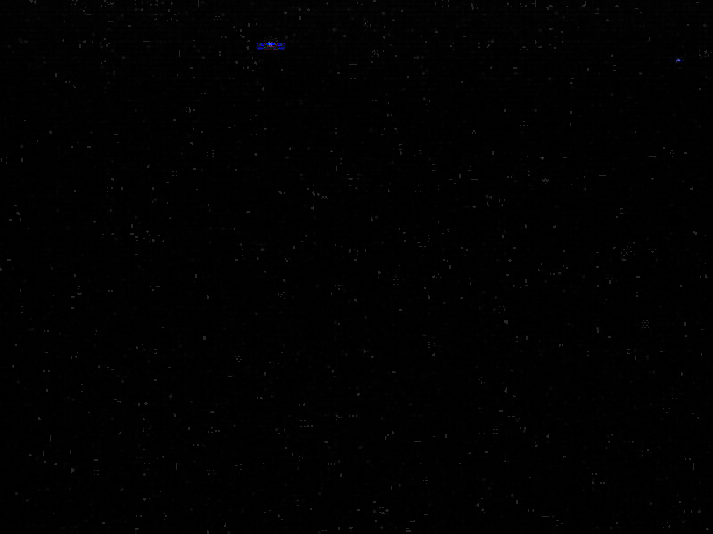
From empirical observations, time-varying noise in digital cameras visually appears to be random color variations across the surface of the image. The level of this noise is related to the ISO setting of the digital camera. This is usually configurable through the camera.
The ISO series settings represent a tradeoff between camera sensitivity and image noise levels. As the ISO setting is increased, the level of image noise increases, but one can reduce the exposure time (assuming all other settings kept equal). Reducing the ISO setting will produce higher quality images, but a longer exposure time is required. This might be unacceptable for very fast subjects or for low-light situations.
The effect of the noise demonstrated by the image series below. From left to right, these images show noise levels at ISO 50, 100, and 400 for the Canon Powershot S1 IS.
Measuring the characteristics of inexpensive consumer digital cameras presents several challenges. Ideally, we would like to break down the image pipeline as finely as possible, isolating sources of noise through each stage of the pipeline. However, most cameras only output the final, processed image data.
When characterizing high-end digital cameras and cameras for scientific applications, generally one can obtain digital values read directly from the CCD or CMOS image sensor.
CCD image sensors have a linear response. That is, for each photon absorbed by the CCD, one electron is produced. However, amplifiers in the camera system may cause the output signals to be nonlinear.
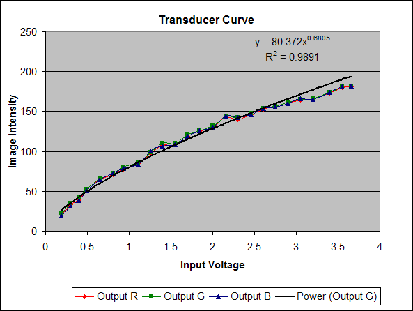
In the case of final images (meant for display), an additional, intentional nonlinearity is introduced. The image intensity values are generally adjusted so that images will be perceptually accurate on common display technologies, such as a cathode ray tube (CRT). The function that describes the mapping from digital CCD values to final image intensity is often called the transducer function and generally follows the form
y = A * x gamma
where x is the digital CCD value, y is the final image intensity, and A and gamma are constants. A may an arbitrary real value, and gamma is ususally somewhere within the range 0.0-1.0.
To properly infer CCD signal levels from a final image, we must apply the inverse of the transducer function to each image pixel in the final image. Since the image intensity scale is essentially arbitrary, we may ignore the constant A and simply set A=1.
Digital cameras use white balancing algorithms to remove color cast from images. We omit the details for the reasoning behind white balancing. The net effect is that the white balancing algorithm performs a linear transformation on the three color values of each pixel.
Ideally, we would like to know what this linear transformation is, but this is very difficult without some fairly involved testing. All current digital cameras have an automatic white balancing mode, which adaptively tries to adjust image intensity to have a perceptually balanced color quality. Most digital cameras also have several settings that allow you to specify the illuminant. We try to choose one of these more specific white balance settings, so that the camera white balance processing will presumably be more nearly constant from shot to shot. Unfortunately, there is no guarantee that this is definitely the case.
JPEG compression introduces a small (presumably imperceptible) amount of noise into the image through the compression process. JPEG compression involves taking 8x8 blocks of pixels in the YCbCr color space, transforming them into the frequency domain, and then quantizing the data to improve compressibility. High- frequency coefficients are quantized most heavily, meaning that relatively more high-frequency noise is introduced into the image than low frequency noise.
There is also a significant amount of noise due to the segmentation of the image into 8x8 blocks. Since each block is processed independently, discontinuities occur along the block boundaries. Taking an image of the noise variance of the blue channel and its 2D Discrete Fourier Transform:
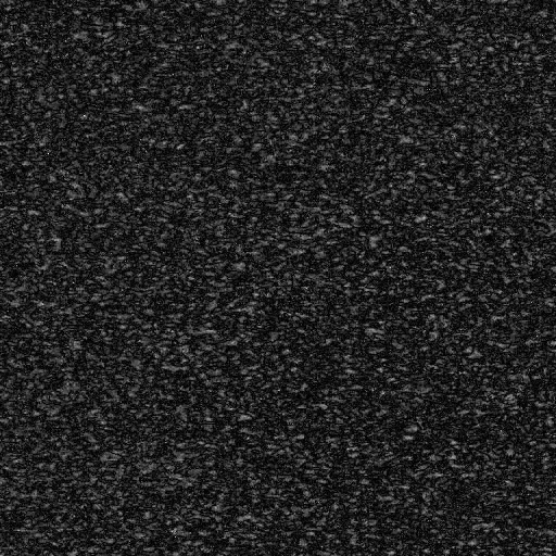
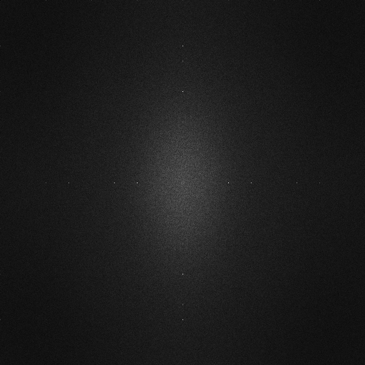
Image of noise variance and 2D FFT of noise variance (click to enlarge)
The image of the noise variance does not show any particular spatial structure, but the 2D FFT of the noise contains an interesting feature. There is a distinct, periodic pattern of peaks along the vertical and horizontal center axes of the FFT. These peaks correspond to artifacts along an 8x8 grid in the image. To demonstrate this, we generate a pattern of random noise along a grid with 8x8 spacing, using a matlab script:
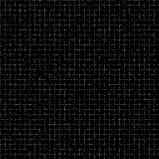
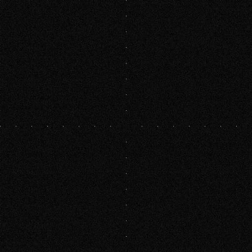
Image of simulated block artifacts and 2D FFT of simulated block artifacts(click to enlarge)
The images are not precisely the same, but this most likely has to do with the other components in the actual image. However, the similarity is enough to explain this feature seen in the FFT of the noise variance.
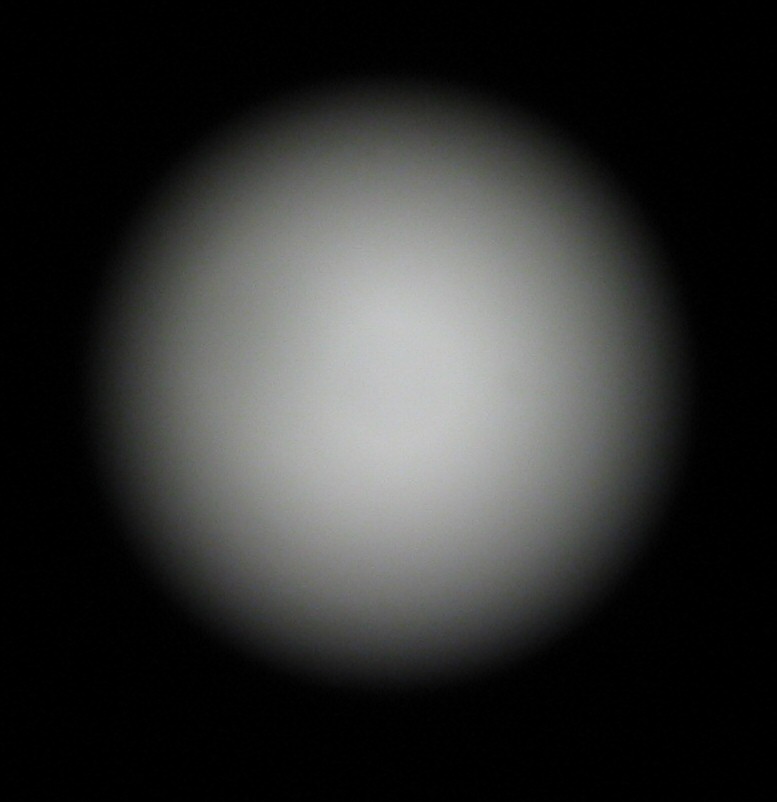
Purpose: Quantify the relationship between input light level and final image intensity.
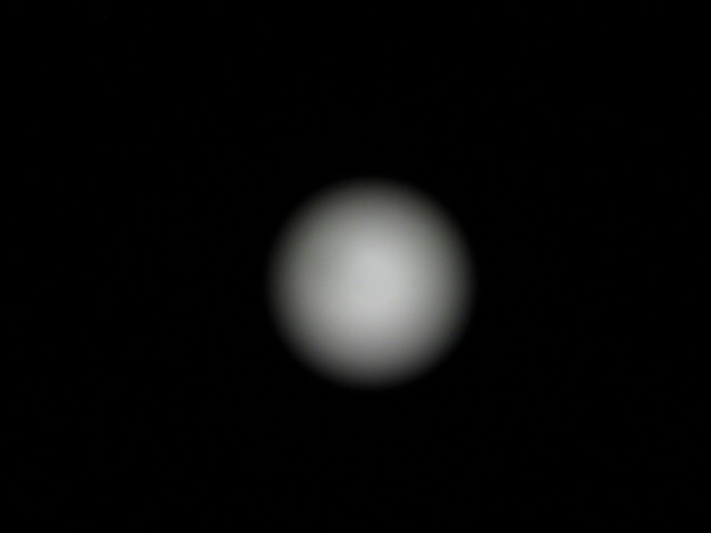
Left: Resized version of an image from Optoliner.
Right: Full-size image from Optoliner, cropped.
For this test, we take a series of images of a light source of known intensity (in candelas). We aim the camera at the Optoliner, and set the lens focus to infinity, since it is not possible to remove the lens. We then take three shots at each light intensity level, and record the intensity setting reported by the light's power supply. Exposure is at about 0.6 seconds, F/2.8, ISO 50. You may view the EXIF data of the above images. We use the following Matlab script to average the three images and compute a consistent intensity for this image.
The test images from the Optoliner take the form of a circle of radially symmetric, but non-uniform, intensity. Therefore, we find the centroid of the circle, and take the average intensity of a 100x100 patch around this centroid. This should give a reliable mean intensity in the presence of noisy camera data.
Purpose: Observe the image noise due to dark current.
For this test, we take a series of images under no illumination -- that is, with the lens cap in place.
Since dark signal levels are quite low, it is not necessary to apply the inverse transducer function to the image data.
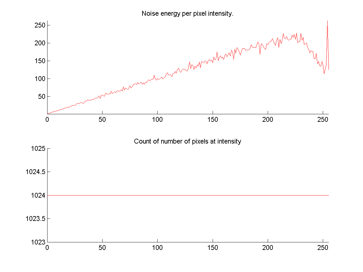
Purpose:: Observe the relationship between signal level and noise variance.
For this test, we aim the camera at a test target that causes the final image intensities to have a maximal dynamic range. We then take a sequence of images, measure the sample mean, and compute the variance of each sample image from the Sample.
To maximize the dynamic range of the image, we aimed the camera at a high-contrast LCD monitor (Samsung 172X, 500:1 contrast), and displayed a linear gradient image across the screen, as shown below.
As a precaution against introduction of artifacts from the discrete red, blue, and green sub-pixels of the LCD, one must manually defocus the camera to infinity. This increased pointspread ensures that color artifacts and moire patterns from aliasing will not occur. It is important that the camera have a manual focus control, as most autofocusing algorithms will have trouble attaining a consistent focus lock on the gradient image.
As a side note, the gamma of the monitor should not be an issue, as we are only trying to get an approximately flat, continuous histogram that has data at all intensity values. The precise quantity of each intensity value need not be precisely the same.

Several consumer digital cameras were put under test. The camera of primary interest is the Canon S1 IS. Other cameras were included to watch for any unusual noise characteristics.
| Make/Model | Release Date | MSRP at Release Date (USD) |
Average Retail Price, March 2005 |
Sensor Type | Max Resolution | Image Output |
| Canon Powershot S1 IS | 2004-02-09 | $499 | $361 | CCD | 2048x1536 | JPEG |
| Canon Powershot S30 | 2001-10-01 | ? | N/A | CCD | 2048x1536 | JPEG or RAW |
| Canon A70 | 2003-02-27 | $449 | $199 | CCD | 2048x1536 | JPEG |
| Canon A80 | 2003-02-20 | $499 | $317 | CCD | 2272x1704 | JPEG |
| Nikon D70 Outfit | 2004-01-28 | $999 | $1150 | CCD | 3008 x 2000 | JPEG, Raw sensor (NEF) |
| Nikon Coolpix 4300 | ? | $399 | ? | CCD | 2272x1704 | JPEG |
| Logitech Quickcam Pro 4000 | ? | $99 | $99 | CCD | 1280x960 (tested at 320x240) | JPEG |
Source data: megapixel.net, DCRP, Logitech
In the interest of conserving bandwidth and disk storage, most of the actual sample image data is kept offline.
The nonlinearity procedures produced the following data:
The following table summarizes some of the results of tests performed to assess camera noise.
In the column Matlab Output, I have linked to a text file summarizing the noise statistics generated by the matlab script. In the first part of the file, each image is summarized by some lines such as:
stats =

    0.0043    0.0045    0.0061    0.0046
    0.0676    0.0755    0.2329    0.0793
         0         0         0         0
    6.0000   14.0000   58.0000   14.1300
The rows describe, in order, mean, standard deviation, min intensity, and max intensity. The columns correspond to the red, green, blue, and greyscale channels. Greyscale is computed using the luminance formula L = 0.3*R + 0.59*G + 0.11*B.
In the second section details, for each image, statistics such as
canon_s1is/darkcurrent\Capture_00050.JPG
Norm Covar -- R-G , R-B, G-B, RGB
0.017662 0.017593 0.017656 0.015414
Covar -- R-G , R-B, G-B
0.986157 0.915273 0.921777 0.015414
Noise RGB
 0.017974 0.017847 0.020557
The first line is the name of the image file read. The third line details the normalized covariance (sometimes called correlation). The fourth line is the covariance among pairs of channels. In the correlation and covariance lines, ignore the fourth value. The fifth line details the average noise energy in each of the R, G, and B channels. (Similar to variance).
Matlab routines| Data Set | Samples Taken | Sample | Matlab Output | Original Resolution |
| Canon S1IS Dark Signal Nonuniformity - ISO 50, 1" exposure | 100 |
Sample Noise Sample |
Output | 2048 x 1536 |
| Canon S1IS Flat Fill (ISO50) | 10 | Sample Noise Sample |
Output | 2048 x 1536 |
| A70 Flat Square of Macbeth Chart (ISO50) | 8 | Sample Noise Sample |
Output | 2048 x 1536 |
| A80 Flat Square of Macbeth Chart (ISO50) | 11 | Sample Noise Sample |
Output | 2048 x 1536 | S30 Flat Fill (RAW, ISO 50) | 51 | Sample Noise Sample |
Output | 2048 x 1536 |
| Quickcam Image | 51 | Sample Noise Sample |
Output | 2048 x 1536 |
Gradient images were processed with different matlab routines. This code isn't particularly well-commented, but it should give an idea of what techniques I tried to use:
| Data Set | Samples Taken | Sample | Matlab Output | Original Resolution |
| Canon S1IS Intensity Gradient - LCD (ISO50) | 30 | Sample | SNR Plot | 2048 x 1536 |
| Canon S1IS Intensity Gradient - LCD (ISO100) | 30 | Sample | 2048 x 1536 | |
| Canon S1IS Intensity Gradient - LCD (ISO200) | 30 | Sample | 2048 x 1536 | |
| Canon S1IS Intensity Gradient - LCD (ISO400) | 30 | Sample | 2048 x 1536 |
These plots compare SNR levels at various signal (image intensity) levels.
For the most part, the SNR data for the image data has a similar profile to that of pure photon shot noise, except near the high intensities, where SNR increases substantially. This increase in SNR corresponds to the decrease in variance at the high intensities seen in the third plot, variance vs. intensity. The reason for the drop in variance is unknown. Simulations of photon shot noise indicate that the variance ought to increase as signal level increases, except for a very small interval near the saturation value. [1]
The dark signal nonuniformity (DSNU) experiments show that typical DSNU levels are well below 1 ADU, even for exposure times as long as 1 second. So we see that DSNU is not a major component of image noise.
The
Given the above data, it is likely that the major source of the noise in typical images is mostly shot noise.
We return to the series of images at various ISO settings. Comparing the ISO 50 to ISO 400 shot, one may perceive a slight shift in the tone of the white wall. In the ISO 50 shot, the wall appears to take on a warm (more red) tone, whereas the ISO 400 shot appears to be cooler (more blue/green).
Left to Right: ISO 50, ISO 100, ISO 400
Data shows that the noise variance in the blue channel is higher than that of the red channel, but there is no evidence that the noise in the blue channel is biased toward being more intense (which would cause the image to actually be more blue).
We have a few hypotheses as to what is causing this effect. One is that the human visual system detects and filters the red noise readily, while confusing blue noise with actual blue signal from the image.
At a given spatial frequency, the human visual system is more sensitive to red variation than to blue variation. Therefore, it is likely that we would perceive more noise in the red channel than the blue channel, given equal noise variance. It is quite likely that we would only perceive the low frequency component of the blue noise. However, from a mathematical point of view, low frequency noise may as well be actual image signal. It seems reasonable that we would "classify" the blue noise as image signal and thus think that the image is actually more blue than it actually is.
The above hypothesis relates to the human white balancing phenomenon. However, there is also the possibility that the camera's white balancing algorithms might be confused by the noise. Similar arguments as above apply, except that we have no evidence as to what parameters affect its white balancing algorithm.
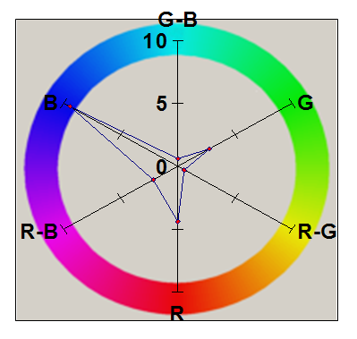
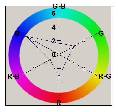
In the section Noise Data Sets, we presented some raw data on the levels of noise variance in the final images acquired. It is important to note that the Noise Sample images are not the actual intensities of the noise, but rather the variance (meaning the square of the absolute value) of the noise. A brighter pixel intensity indicates that there is a strong deviation (either positive or negative) from the mean value of that pixel.
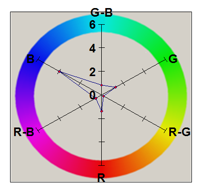
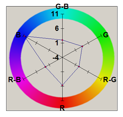
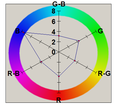
The radar plots below give an interpretation of the spatial noise variance samples. They quantify the average variance of the red, green, and blue channels, as well as the covariance of pairs of channels. Note that all channels have positive covariance. While it is not possible to know exactly what processing steps occur inside the camera, it seems likely that these positive covariances are due to the interpolation of pixels in the CCD color mosaic. The wide spatial patterns of the blue and red channels are evidence of this, since the Bayer mosaic pattern has relatively fewer red and blue pixels, compared to green.
| Noise Variance | Var/Cov Plot | |
| Canon S1 IS |  |
 |
| Canon S30 | 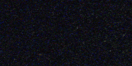 |
|
| Canon A70 | 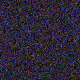 |
 |
| Canon A80 | 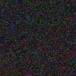 |
 |
| Logitech Quickcam Pro 4000 |  |
 |
There are several well-known techniques for removing noise from images. We summarize a few of these below:
Noise removal algorithms have become common in image processing software. Jasc Paint Shop Pro 8 contains an algorithm it calls "edge-preserving smooth." It is possible that this algorithm is the bilateral filter, but there is no conclusive evidence for this.
There is also software dedicated to the purpose of removing image noise. A comparison of these noise removal programs is beyond the scope of this project, but I will briefly describe one such program, Neat Image.
The generic algorithms described do not explicitly take the image noise statistics into account. Neat Image utilizes device noise profiles, which describe the character of noise of specific cameras. This allows the noise removal algorithms to remove noise without removing as much image signal.
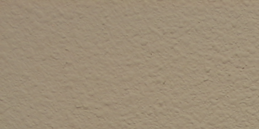
The program does an excellent job of removing noise, as seen in the test image at taken at ISO 400, below. Some points to notice are that the algorithm does an excellent job of preserving the sharpness of edges and of generally recovering perceptually accurate image color, compared to the original image color.

Left: ISO 400 Unfiltered Image
Right: ISO 400 Image, Filtered
[1] A. J. P. Theuwissen, Solid-State Imaging with Charge-Coupled Devices, Solid-State Science and Technology Library (Kluwer Academic, Boston, Mass., 1995)
[2] Brian A. Wandell, Foundations of Vision, Sinuer 1995.
[3] C. Tomasi , R. Manduchi, Bilateral Filtering for Gray and Color Images, Proceedings of the Sixth International Conference on Computer Vision, p.839, January 04-07, 1998.