Implementing
Image-Processing Pipelines in Digital Cameras
Jong B. ParkDepartment of Electrical Engineering, Stanford University 9:15 AM, March 12, 2003 |
Introduction
A
general image-processing pipeline in a digital camera
can be mainly divided into two steps: Sensor
measurements à 1. Spatial Demosaicing è 2. Color Correction à
Gamma correction Depending
on the method of each step, the final image quality can significantly vary. However,
image-processing algorithms in a digital camera is embedded in a chip, and we
cannot modify them to test or improve the final image quality. Therefore, in this project, I manually
applied each image-processing steps in order to understand, and potentially
improve, the final image quality of a digital camera. This
report provides intuitive understandings on the design and trade-offs of
spatial demosaicing and color correction (or color balancing) techniques, and
their effect on the final image quality. Note: PowerShot G1 from Canon, which has the raw
sensor-data mode, was used. The CMYG
sensor matrix was composed of approximately 2000 x 1500 pixels. More details
are listed at http://www.dpreview.com/reviews/canong1/.
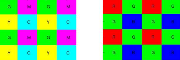
-------------------------- Figure
1 shows Color Filter Array (CFA) pattern for the digital camera used in this
project. CFA covers the sensor
matrix, and each pixel measures light with a color represented by the filter.
Figure 1. Color Filter Array
(CFA) Pattern: CMGY pattern used in this
project, and typical Bayer pattern for RGB. The pattern is repeated
covering the whole sensor matrix. The
recovery of full-color values at each pixel, i.e., the recovery of full-color
image with the same spatial resolution of a pixel, requires a method called
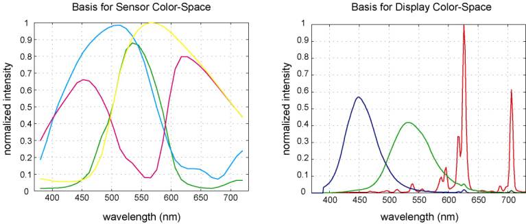
color interpolation or color demosaicing algorithms. General
purpose of a color correction matrix (or color balancing matrix), is to
convert the measurements from sensor color-space to display color-space, which
can be either sensor RGB to display RGB, or sensor CMYG to display RGB (see
Fig. 2). The trade-off here
will be between noise and color error in the transformed color-space
[5]. Here, our color correction
matrix Cc will be a 3x4 matrix, which converts sensor CMYG
values to display RGB values.
Figure 2. Typical CMYG and
phosphor-RGB spectral waveform.
Equation 1. Color
Correction or Color Balancing Equation. ( G, M, C, and Y are 2000
x 1500. R, G, and B are 2000 x 1500 ) In Eq. 1, if we think of m x n x l dimension of
3D matrix as vertical x horizontal1 x horizontal2, then the color
correction can be thought of as performing linear combinations in vertical
direction at each horizontal location, i.e., at each pixel. The spatial demosaicing can be thought of
as linear operation (in fact, it is low-pass filtering; details will be
discussed later) in the horizontal plane.
Therefore, the order of color correction and spatial demosaicing
operation can be interchanged. For presentation purpose, I will first discuss “Step II – Color Correction,” whose results does not require sophisticated demosaicing algorithms to visualize, whereas “Step I – Spatial Demosaicing” requires decent color correction matrix to display the results. Note: typical gamma value of 2.2 was used to do gamma correction
for all results presented here. Step II – Color Correction
To
design color correction matrix Cc, we have to know the spectral
waveform of the sensor (i.e., response-curve of the sensor CFA) and spectral
waveform of display phosphors, similar to the ones shown in Fig. 2. Although, display phosphors may vary, the spectral waveform
given in Fig. 2 can be a good approximation compared to the variations in the
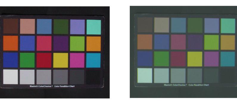
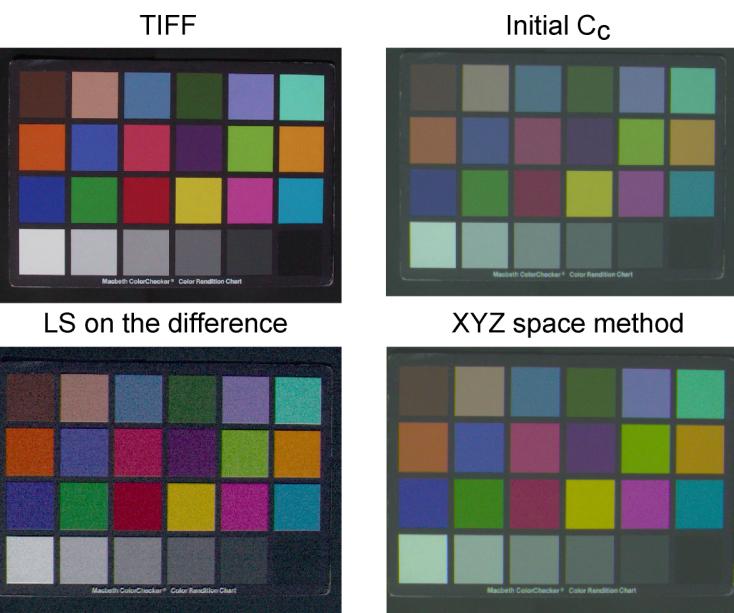
sensor response-curve among different digital cameras. Figure 3 shows the initial result compared
with the direct TIFF output of the digital camera.
Figure 3. Macbeth
Color-Checker Board: (left) direct TIFF output
from digital camera, (right) raw-data color
corrected with initial Cc; Initial Cc.
produced poor color contrast. As
shown in above figure, initial Cc, based on assuming simple
CMYG response-curve of the sensor, could not be used. Therefore, it was necessary to measure
of spectral response of CMYG CFA of the sensor. One common method of approximating the spectral response of the
sensor, R, using the color-checker board is to solve below linear
equation for R. (Although
we have to characterize the sensor noise and the light source, I focused on
measuring the response since we can assume dominated noise as poisson and can
use sun light to approximate the 6500K white illuminant D65.)
Equation 2. Linear
equation for approximating the sensor response, R, using color patches. S represents spectrometer
measurements of 24 color patches, and D represents the digital camera raw
measurements of each CMYG sensors. The number of spectral samples was 101 in the visual frequency range.
We
measured spectrums of Macbeth Color-Checker Board with 24 color patches on sunny
day outdoor between 12 to 2 pm, in order to acquire approximately 6500K white
illuminant D65, using our digital camera (Canon PowerShot G1) and
the spectrometer that provides 101 spectral samples in the visual frequency
range. For the digital camera, white
balancing was set to daylight, and we acquired total of 21 pictures (7
pictures with 3 different exposure settings). 4 spectrometer measurements
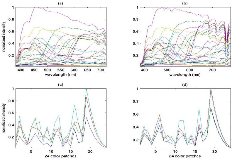
were acquired. Figure 4 shows the
average of the measurements shown with the ideal responses from the simulation.
Figure 4. Spectral
Responses of Macbeth Color-Checker Board: (a)
simulated spectral responses of ideal color-patches, (b)
actual measurements using spectrometer with the real color-checker, (c)
simulated CMYG sensor measurements with responses shown in Fig. 3, (d) actual CMYG sensor
measurements of the real color-checker board. Solving
Eq. 2 with pseudo-inverse gives a least norm solution. However, in the presence of the noise, we have to consider the
condition number of k, which is the measure of
the sensitivity of the solution to noise (see Eq. 3).
Equation 3. Condition
Number of a linear equation y = Ax where
and s(A) = singular value of A. Large k(A) means the estimation x will be more sensitive
to noise in the measurement y. Note that the condition
number is the measure of “geometric anisotropy” (thus k = 1 for an orthogonal matrix). Our
initial condition number k(S) is very large because the
24 color patches were illuminated with the same light, meaning that 24
vectors of 101-dimension were far from being orthogonal to each other. Even in
simulations with the ideal S, the estimation of R
was very sensitive to the noise (see Fig. 5). The k(S) was 2e3 for the simulation
and 1e4 for the actual measurements.
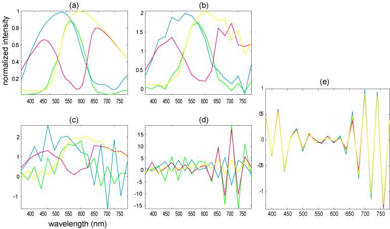
Figure 5. Sensor Response
Estimation. (a)
Simulated results with no noise, (b)
with noise level of 0.003%, (c) with noise level of 0.03%, and (d) with noise
level of 0.3%. (d)
actual results from the measurements; the worn-down color patches may have produced the similarity in the
response (e). One
way to reduce k(S) was to reduce the sample
number of spectral wavelengths, i.e., reducing the column of S. Although this provided more robustness to noise in
the simulation, no significant improvement was visible the actual estimation even
with the spectral sample number of 3.
The possible reason can come from the fact that noise level is much
higher than the simulation, and that S also contained noise, which is
not the case in the simulation. For
the comparison of spatial demosaicing algorithms, better color correction
matrix Cc was still needed. The next method I tried was manually increasing the
saturation of the colors, i.e., increasing the color contrast, in the
intermediate color space, the standard XYZ color space [6]. CMGY color space of the sensor à XYZ color space à RGB color space of the display After
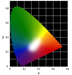
estimating the white points from one of the color patches, I amplified the
distance of each color in the chromaticity plane (Fig. 6) with respect to the
white point. (Note that doing this in
regular XYZ space may fail because white point vector will have the largest
norm, which means that amplifying the distance with respect to white points
result in overall shift into one of the corners in the chromaticity plane.)
The result is shown in Fig. 7.
Figure 6. Chromaticity
Diagram. Note that this is similar
to projection of XYZ space onto X+Y+Z = 1 plane.
Figure 7. The result from
Color Correction Matrix Estimation using XYZ space method,
and Least Squares (LS) on the difference method. The color contrast increased
but at the same time, noise was amplified. Even
though XYZ space method improved our initial Cc, the poor result
suggested for another approach. Above
two methods, solving linear equations from the spectral measurements of color
patches and XYZ space method, can be implemented independent of existing
image-processing pipelines. However,
since we have already working image-processing pipeline that provided TIFF
output, we can estimate the error term in Cc.
Equation 4. Linear
equation for estimating the error term, DCc,e, which can
be solved by simple Least Squares (LS); see Eq. 1. The
result by using the difference from the TIFF output was shown in Fig. 7. Note
that the result was using only one image of the color-checker from the
digital camera. Step I – Spatial Demosaicing
The previous
class project by Chen [1]
focused on implementing various demosaicing algorithms with RGB Bayer pattern
[2]. Typical RGB demosaicing
algorithms can be categorized into two groups: non-adaptive and
adaptive. Non-adaptive methods include
Nearest Neighbor Replication (NNR), Bilinear Interpolation (BL), Cubic
Convolution, Smooth Hue Transition, etc., and adaptive methods include Edge
Sensing, Variable Number Gradients, Pattern Recognition, etc. However, the analysis of the spatial
demosaicing algorithm has been based on image-domain perspective rather than
Fourier domain perspective. In general, any
operation or processing performed can be analyzed in Fourier space. Any spatial
demosaicing or interpolation algorithms can be though of as low-pass
filtering the aliased spectrums, due to undersampling, in the Fourier domain.
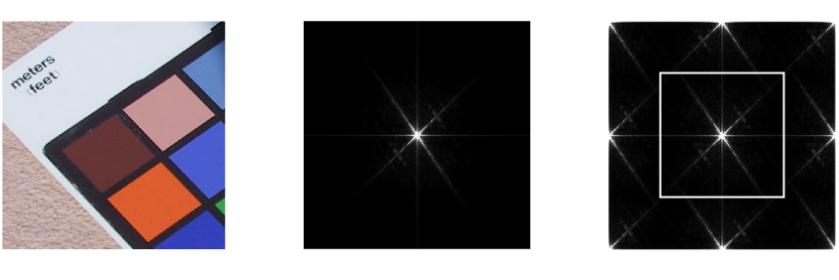
Figure 8. 2D
Spatial-Frequency Spectrum in Fourier-space: (left) original image in
image-space, (middle) magnitude image
of 2D-FT on fully-sampled image, (right) magnitude image of 2D-FT on under-sampled image (i.e.,
Cyan pixels) with typical low-pass
filter (with cut-off frequency of ¼ Nyquist frequency) shown as rectangular
box. Horizontal and vertical lines
crossing the center are possibly due to line-pattern noise in the sensor. Most non-adaptive
demosaicing methods for RGB Bayer pattern are equivalent to using low-pass
filters that has effectively low cut-off frequencies. However, NNR is equivalent to using rect
kernel, which has sinc shaped low-pass filter that provides poor stop-band
characteristics; moreover, uni-direction NNR has a low cut-off frequency
in the direction of replication but no low-pass filtering is performed in the
perpendicular direction, which results in severe high spatial frequency
aliasing artifacts (see the results in [1]). Adaptive
method, which uses local spatial information to decide different demosaicing
algorithms, is equivalent to using different-sized convolution kernels of
low-pass filters at different spatial locations, namely, adaptive filtering. The
advantage of Fourier perspective is that we can directly control the trade-off
between noise and spatial-resolutions. Also,
various digital-filter-design techniques, which have already been extensively
researched, can give us better understandings and more flexibility in
designing demosaicing algorithms. The trade-off in computational cost can be
regarded as the trade-off between FIR filter length and ringing (or error) in
the pass-band of a low-pass filter. Recently,
Fourier domain approach was presented [4].
They use normal low-pass filtering for the luminance channel but apply
high-pass filter to use aliased spectral-islands instead of the central
spectral-island for chrominance channel (see Fig. 2). However, the central spectral-island
contains the information in the aliased spectral-islands because they are the
replication of the central islands due to under-sampling. Instead
of converting the RGB-Bayer-pattern demosaicing methods to CMYG pattern in
Fig. 1, which has not been not researched extensively, Fourier domain
approach was used to solve CMYG demosaicing problem, i.e., solving the
spatial demosaicing problem by designing a 2-dimensional low-pass FIR
filter with well-known digital filter techniques [3]. I applied the same low-pass filter for all
four color (CMGY) channels. The results from digital filter approach, and from Nearest Neighbor Replication and Bilinear Interpolation methods similar to the one with RGB Bayer pattern are shown in Fig. 9.
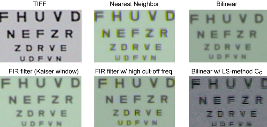
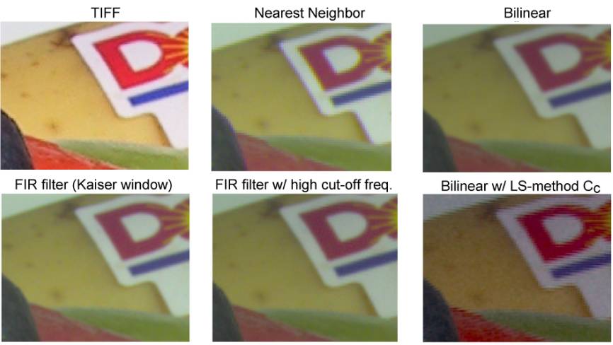
Figure 9. Spatial
Demosaicing Results I.
Figure 10. Spatial
Demosaicing Results II. FIR filter with Kaiser Bessel window (b = 8) was using cut-off frequency of 0.25 (left figure) or 0.35 (middle figure) Nyquist frequency; note that the maximum cut-off frequency possible is 0.5 Nyquist frequency where Nyquist frequency represents 1/pixelwidth. Nearest Neighbor Replication method with CMYG pattern cannot be done in uni-direction (see Fig. 1). Therefore, the result is better than the one shown in previous work [1]. The direct TIFF output looks sharper than FIR filter results (see left figures in Fig. 9 and 10). The possible reason is the sharpening operation in the embedded image-processing pipeline in the digital camera, which amplifies higher frequency components after the demosaicing (i.e., low-pass filtering) process. Note that the possible anti-aliasing filter in front of CFA may have suppressed higher frequency components before the sensor measurements because it is hard for physical anti-aliasing filter to have flat response in the low-frequency pass-band. Conclusions
Optimal
spatial demosaicing and color correction methods are essential for designing
image-processing pipelines in digital cameras. As we have seen, depending on the color correction matrix and
spatial demosaicing algorithms, the final image quality can significantly
vary. To
achieve good color correction matrix, the spectral response information of
the sensor is crucial. In the future
work, using larger number of color patches or larger number of color
checker measurements to reduce the condition number of the linear
equation, and/or using brute-force adjustments of 12 = 3x4 elements in
the color correction matrix can be done.
Moreover, the accurate characterization of the sensor noise may be
necessary. To
improve spatial demosaicing algorithms, the digital sharpening filter
can be implemented. Moreover, it the
computational time is important, one can directly use narrow Kaiser window
or narrow Gaussian window as a convolution kernel instead of sinc kernel. The Kaiser or Gaussian window is widely
used in various 1D- and 2D-filtering applications due to its controllability
of both domains and the property of fast decay. References
[1]
Chen,T., “A study of spatial color
interpolation algorithms for digital cameras,” Psych221/EE362
project, winter 1999. [2]
Bayer, B.E., “Color imaging array,” U.S. Patent 3,971,065 [3]
Oppenheim, A.V., and Schafer, R.W., “Discrete-time signal processing,”
Prentice Hall. [4]
Alleysson, D., et al., “Color demosaicing by estimating luminance and
opponent chromatic signals in the Fourier domain,” IS&T/SID Tenth Color
Imaging Conference, 2002. [5]
Barnhoefer, U., et al., “Color estimation error trade-offs,” ulrichb
AT stanford DOT edu. [6]
Wandell, B.A., “Foundations of vision,” Sinauer. Appendix I
MATLAB
source codes do_all.m : main project file. crw600.exe : dos program for converint CRW raw-files to
PPM files. getraw4.m : reading PPM files. LSdiff.m : forming linear equation variables for Least
Squares on the difference method for color correction. do_resp.m : extracting spectrometer data and solving
Least Norm problem. segment_patch.m : for region of interest
segmentation. MATLAB
data files whiteX0Z.mat :
white patch data xyz_phos_tutorial.mat : XYZ color-matching
functions new_color_corr.mat : the result of XYZ-space
method for color correction. Please contact me at below email address for other source codes and
data-files. THANK
YOU FOR VISITING THIS WEBSITE !!! |
Jong Buhm Park (piquant AT mrsrl DOT stanford DOT edu)
Research Assistant / PhD student
Magnetic Resonance Systems Research Laboratory
Department of Electrical Engineering
Stanford University