Perceptual Color Image Segmentation
project webpage - cs223b & psych221
angela chau + jeff walters
winter qtr 2003
|
|
Perceptual Color Image Segmentationproject webpage - cs223b & psych221angela chau + jeff walters
|
The problem of segmenting images into coherent regions has been a major subject of research in the field of computer vision. Most of the literature written on the topic has concentrated on using texture information to perform the segmentation on gray-scale images. Some researchers, however, have started looking at how color and texture information can be used in combination during the segmentation process, thus introducing the more specific problem of color image segmentation. The term 'color textures' is often used to describe the input images for color segmentation algorithms.
Searching through the major journals over the past few years, it seems that there are a variety of methods people have used to try to solve this problem. Some of these include clustering in various feature spaces, clustering in a color space such as RGB and then merging these clusters in a perceptually uniform color space, using Gabor filters in combination with low-pass color filters, etc. For a more detailed look at two of these other methods, please refer to Appendix 2.
The goal of our project is to investigate one specific approach to the segmentation of color textures, as developed by Mirmehdi and Petrou in [1]. The algorithm they suggested involves using findings from studies of the human visual system and its responses to colors and spatial frequencies of colors as well as the method of multiscale probabilistic relaxation to improve the segmentation process. In general, one would like to have the input to any clustering algorithm closely match the processing that occurs in the human visual system. This helps to ensure that the results are similar to what humans would produce. The use of the SCIELAB paradigm as a pre-processing step to the clustering aims to present the clustering algorithm with color images that mimic the color dependent blurring of texture that occurs in the human visual system.
In [1], Mirmehdi and Petrou developed an algorithm of segmenting color textures through the use of perceptual filters, the formation of initial clusters, and then the application of an iterative process called multiscale probabilistic relaxation to pass information between different scales of the image. The following section highlights some of the key points of the method and walks through an example of how an image is processed by the algorithm. For a more detailed explanation of the technique and its underlying theory, please refer to [1] - [4].
The example image (shown below) is a synthetic color texture created by us for the sole purpose of testing. The textures in the image are taken from the MIT VisTex database.
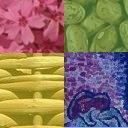 Figure 1: Original Test Image |
S-CIELAB
The first step in the algorithm involves the creation of a perceptual tower from the original image. From results of studies conducted on human vision and [5], we know that the human visual system's responses to color is highly dependent on spatial frequency and high spatial frequencies tend to get more blurred by the eye's optics than lower spatial frequencies. The perceptual tower is an attempt to mimic this dependency.
Using the functions provided in the S-CIELAB toolkit, we construct a series of images that are increasingly blurred by assuming that we're viewing the image from increasing distances. We can think of the tower as how humans might foveate on an image first view from the periphery by first bringing it to the central field of view and then by walking closer to it to look at its details. The following series of images shows the perceptual tower created from the example image (distances are measured in inches):
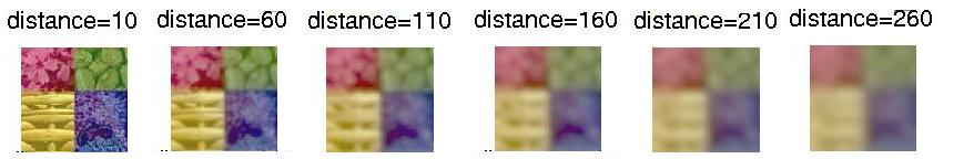 Figure 2: Perceptual Tower |
The filters available in S-CIELAB perform filtering in an opponent color space of Luminance, Red-Green, and Blue-Yellow. Filters are constructed as weighted sums of Gaussian functions and different filters are applied to each plane. For example, the filter for the Luminance plane is very compact compared to that used for the Blue-Yellow plane, corresponding to the differing levels of blurring done by the human visual system.
K-Means Clustering
Before the probabilistic relaxation scheme is applied to the image at the last/coarsest level of the pyramid, we perform a set of pre-processing on this blurred image. The first step is using K-means clustering with a very large K to obtain an initial set of clusters to start from.
Because we would like our clusters to be "blobby" (i.e. little continuous regions in the image) instead of distributed all over the image, we performed K-means using both the pixels' values in the LAB color space as well as their (x,y) coordinates. The initial set of means we chose is simply a randomly distributed set of points in the (x,y,L,a,b) space. During each iteration, each pixel is associated with the cluster "closest" to it. (Distance here is defined as the norm of the difference vector, found by subtracting the pixel's (x,y,L,a,b) coordinates from the mean coordinates). Once all the pixels have been classified, the mean of the cluster is recalculated. This process continues until the mean values stabilize, as determined by a defined threshold.
In our tests, we used very large K values of 10000 or 50000, in the hopes of getting many small clusters that are very likely to actually belong to the same region. The following image shows the resulting clusters after K-means clustering:
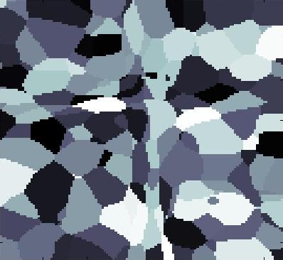 Figure 3: After K-Means Clustering |
(Note: In the above image, each "blob" corresponds to a separate cluster and blobs of the same color are actually different clusters. We had trouble finding a colormap with enough colors to support all the clusters we have.)
Core Clusters
Once we have the large group of small clusters resulting from K-means, we'd like to use them to form an initial set of larger clusters, called "core clusters."
We first iterate through the set of clusters and for each cluster, find all neighbor clusters. If a neighboring cluster has a mean in LAB space that's close to the mean of the current cluster, the two are merged to form a bigger cluster. The "closeness" of the means in LAB space is defined using a threshold value. This merging process stops when it cannot find any more regions to merge.
Next, insignificant clusters are identified by looking at the percentage of the total image each cluster occupies. If this percentage is below another defined threshold, the corresponding cluster is removed from the set.
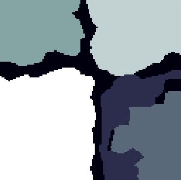 Figure 4: After Cluster Merging |
With this new smaller set of clusters, we next need to calculate probabilities to begin the multiscale probabilistic relaxation process. These probabilities, or "confidences", are calculated according to the formulas presented in [1] for every pixel-cluster pairing. The set of core clusters are then formed by assigning any pixel with confidences over 80% for a cluster to that cluster.
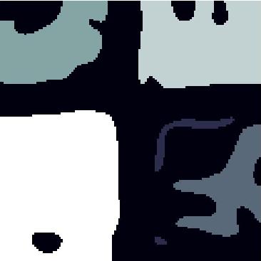 Figure 5: Core Clusters at Coarsest Level |
Probabilistic Relaxation
The technique of probabilistic relaxation, as defined my Mirmehdi & Petrou, creates a framework that allows one to calculate the probability that a certain pixel is a member of a certain cluster. "Relaxation" refers to the iterative approach where probability estimations are made and then updated, iteration after iteration. The probabilities that are estimated at each level are, again, the probability of a pixel being a member of a certain cluster. Once all iterations are complete, a pixel becomes an "official" member of the cluster with which it has the highest probability of belonging.
The iterative nature of the algorithm closely parallels the structure of the perceptual tower that was described earlier. Probabilities are calculated for the coarsest image, and those probabilities are then propagated downward, influencing the probability estimates attained for the more detailed images.
Equation 1 illustrates the general clustering problem. Using the law of total probability and Bayes' rule, this expression can be expanded, and then assumptions can be made that turn the actual computations of the probabilities into a tractable problem. One important assumption is that the probabilities defined for level L are influenced only by the data in that level and also level L+1. Additionally, the probabilities for all pixels are assumed to be independent of one another. This is clearly not true, but the descent down the perceptual tower implies that each pixel's assignment is influenced by its surrounding pixels, thanks to the convolutions that were used to create the perceptual tower.
 Equation 1: General Clustering Problem |
After these assumptions are made, the probabilities can then be explicitly calculated using Equation 2. The second term in the numerator is simply the probabilities that were calculated from the previous level, so no additionally calculations are required. For the first level, this term is calculated as described in the Core Clusters section.
 Equation 2: Formula for calculation of cluster probabilities. |
The first term of the numerator, P(x|theta), and the third term, are calculated as described in the sections below.
P(x|theta)
This term is the probability of a pixel taking on its color (position in the color space) conditioned on its membership in each of the clusters. It is calculated for every pixel in the image. To exactly calculate this term, one would need to know the exact probability distribution function (PDF) of the colors for each cluster. Since colors are represented with three dimensions, this is a three-dimensional PDF.
These PDFs were estimated using histograms. The color space was divided into many cubes, and the number of pixels in a cluster that fall into a given cube was used to then calculate that probability of a certain color's occurrence given membership in a particular cluster.
Q
The Q function itself lacks a simple, intuitive meaning. If is calculated for every pixel in the image, at each level, and for each cluster. Rather, it is the term that contains all terms that are somewhat less intuitive. Referring to Equation 2, one can see that the basic input into Q is P(x|theta), as described above, multiplied with the final probabilities from the previous level.
The key observation regarding Q is the double summation and multiplication. The two summations represent the calculation of a product of probabilities for all possible cluster assignments for every other pixel in the image (aside from the pixel for which Q is being calculated). Clearly, it is impossible to perform this calculation exactly, so some simplifying assumptions must be made. The first simplification is that only a 3x3 region around each pixel will be considered. Thus, we only need to consider the possible cluster assignments for each of the other 8 pixels in the region aside from the pixel in question. Furthermore, not all permutations of cluster assignments need to be considered. It would be highly unlikely, for example, for all nine pixels in a particular region to belong to different clusters. Therefore, a pattern dictionary is created that represents the possible configuration of cluster assignments in an arbitrary 3x3 region in the image. Also, in any 3x3 region, it would be highly unlikely for there to be pixels belonging to more than two clusters, so each pattern contains an arrangement of only two clusters. For some examples of a pattern in the dictionary, refer to the Power Point Presentation.
Putting it all together- Climbing up the perceptual tower
At each level in the pyramid, we calculate all of the above terms as previously described. Then, at each level, pixels are assigned to clusters as described in the Core Clusters section.
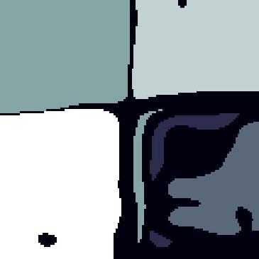
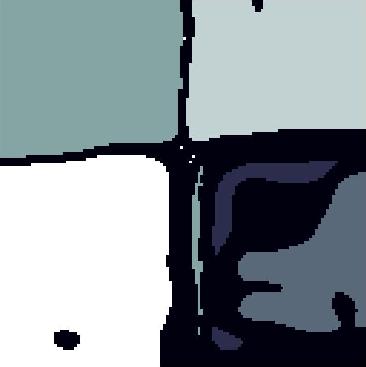
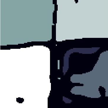
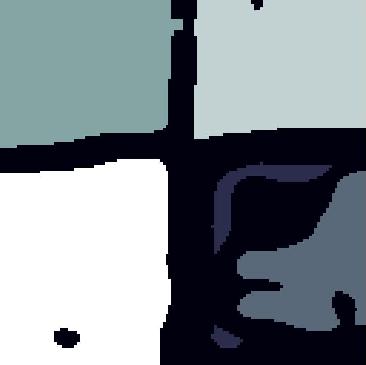
Figure 6 shows this progression:
 |
 |
 |
 |
 |
|
Figure 6: Core Clusters Going Up the Tower (L to R) |
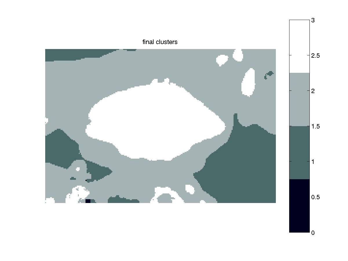
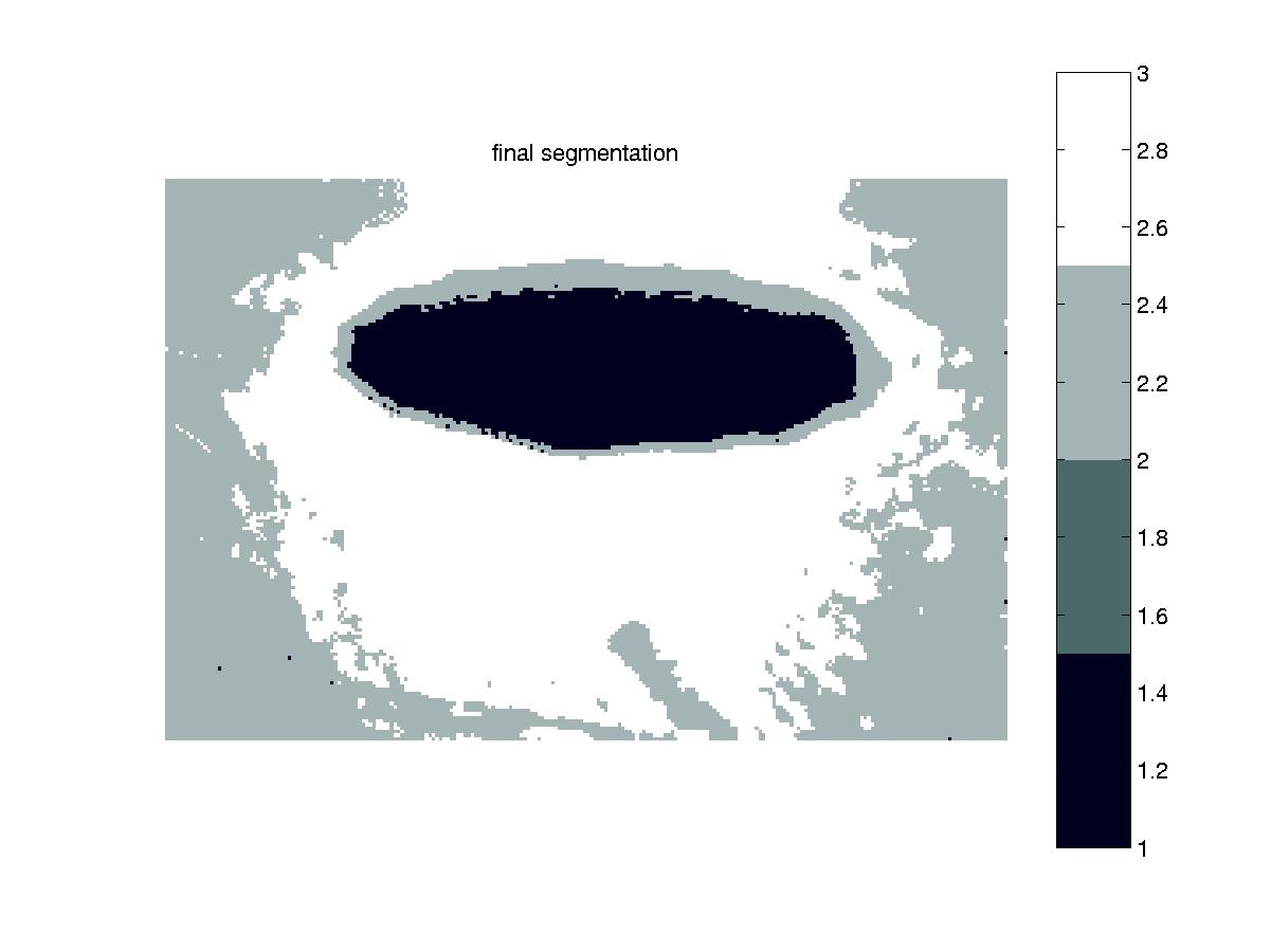
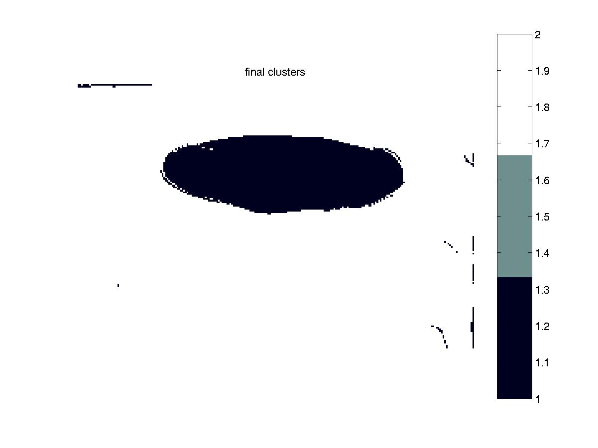
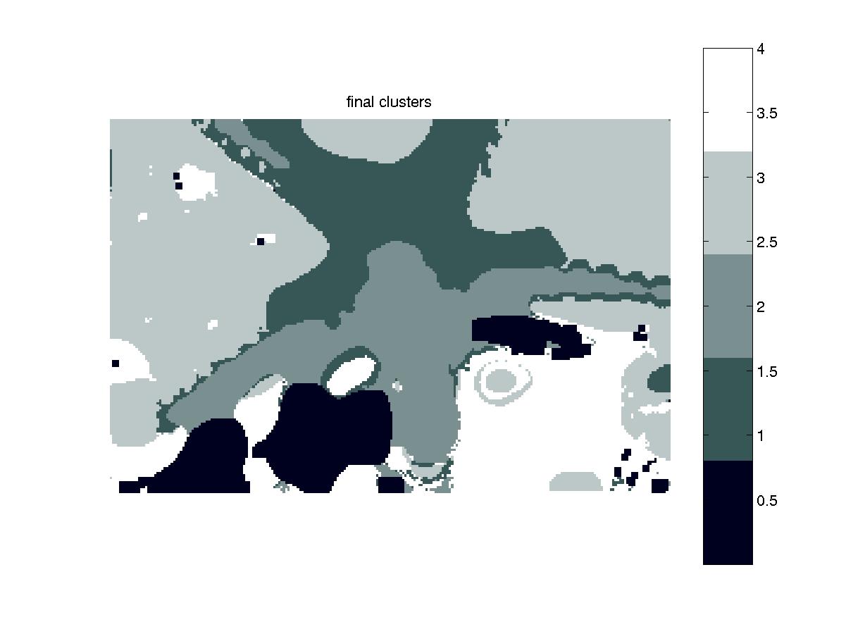
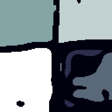
At the last step, the final cluster assignments for each pixel are made, as seen in Figure 7.
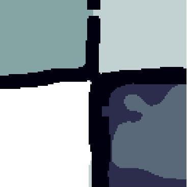 Figure 7: Final Segmentation |
Some of the major challenges we ran into during the project include:
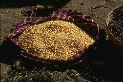
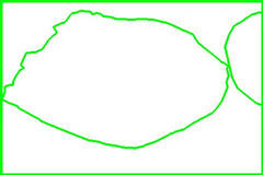
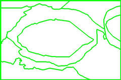
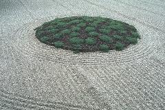
In this section, we present some results of our algorithm on real images. These images are taken from the Berkeley Segmentation dataset. To sanity check our results, we also present two representative segmentations done by human users taken from the dataset website. Although segmentations between users vary, we have tried to choose the segmentations which contain the "least common denominator" amongst the set.
To save space, we do not present any intermediate results for these images. If interested, please contact either Angi or Jeff.
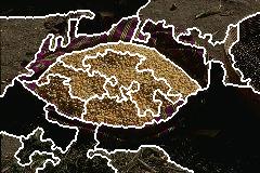
Grain Image (initial K=10000):
|
|
|
|
Grass Image (initial K=10000):
|
|
|
|
Grass Image (initial K=50000):
|
|
|
|
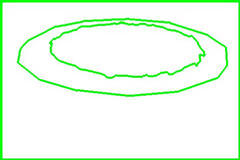
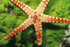
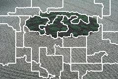
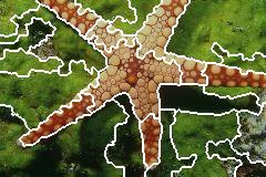
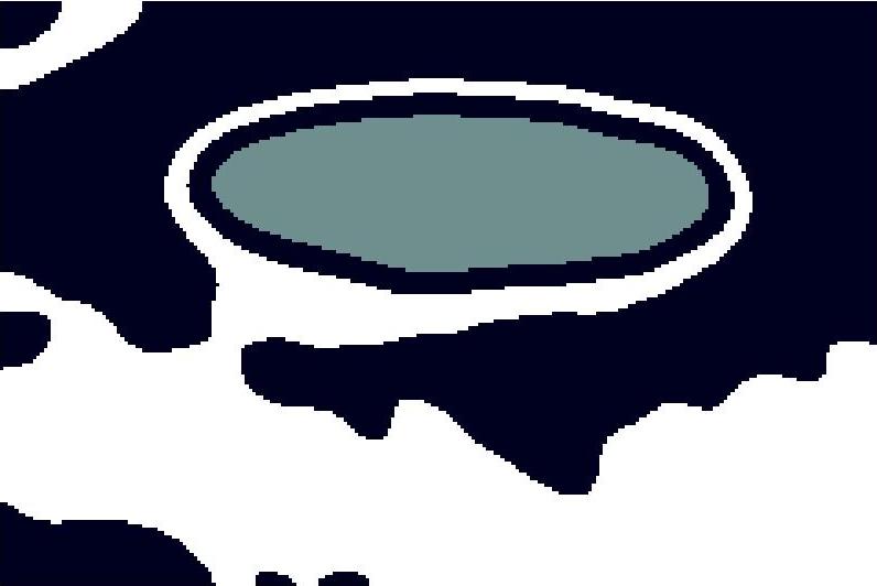
Starfish Image (initial K=50000):
|
|
|
|
We can make several observations from the above set of data. First, the segmentation algorithm is quite sensitive to the initial value of K, as can be seen from the different segmentations resulting from two different K values for the grass image. While our algorithm seems to do relatively well in discerning which textures would be considered a single region by humans, it seems to be weaker in accurately localizing edges. Also, the resulting segmentation images tend to look a bit noisy.
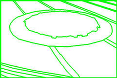
As stated in the proposal, we would like to compare our results with that obtained using another segmentation algorithm. The algorithm we chose is EdgeFlow, developed by Wei Ma and B.S.Manjunath. Using software available from the website, we ran EdgeFlow on the test images above.
Grain Image (initial K=10000):
|
|
|
Grass Image (initial K=10000):
|
|
|
Starfish Image (initial K=50000):
|
|
|
As we can see, EdgeFlow performs very well in accurately finding the edges between regions in the images (as we would expect given its name!). However, it has a tendency to over-segment the image.
While it is quite difficult to objectively judge the quality of our algorithm, as is often the case with image segmentations, we feel that the technique presented by Mirmehdi and Petrou is an innovative and interesting approach to the problem. The strength of the algorithm lies in the fact that it incorporates knowledge of the human visual system in its attempt to perform segmentation "like a person."
Due to time constraints, we did not get a chance to compare our results using perceptual filters with those obtained using the same Gaussian filters on all color planes. Although Mirmedhi and Petrou hinted that the segmentations resulting from this set of filtered images would be very wrong in [1], we feel that this should still be a worthwhile comparison because it will show us the level of improvement gained by using perceptual filters.
We would also like to speed up the performance of the algorithm, and in particular, the K-means clustering done during pre-processing, in order to test out more values of K's and run more tests in general. This can be done by converting the K-means function into C code and linking it into Matlab as a MEX module. Again, due to time constraints, we were not able to implement this enhancement.
[1] M. Mirmehdi and M. Petrou, "Segmentation of Colour Textures," IEEE Transactions on Pattern Analysis and Machine Intelligence, 2(2):142--159, February 2000.
[2] M. Mirmehdi and M. Petrou, "Perceptual versus gaussian smoothing for pattern-colour separability," International Conference on Signal Processing and Communications, pages 136--140. IASTED/Acta Press, February 1998.
[3] M. Petrou, M. Mirmehdi, and M. Coors,"Perceptual smoothing and segmentation of colour textures," Proceedings of the 5th European Conference on Computer Vision, pages 623--639, Freiburg, Germany, June 1998.
[4] M. Petrou, M. Mirmehdi, and M. Coors, "Multilevel probabilistic relaxation," Proceedings of the Eighth British Machine Vision Conference 97, pages 60-69, BMVA Press, 1997.
[5] X. Zhang and B.A. Wandell, "A Spatial Extension for CIELAB for Digital Color Image Reproduction," Proc. Soc. Information Display Symp., 1996.
We have made a zipped copy of our CVS code tree available here.
The literature survey for cs223b can be found here.
The following lists out roughly the division of labor for the project. Please note that Angi is taking both psych221 and cs223b, while Jeff is only taking psych221.
Jeff:
Angi:
Both of us contributed to the content of the project webpage as well as the creation and presentation of the Powerpoint slides.