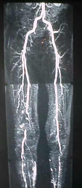
Magnetic resonance (MR) is a rapidly developing noninvasive imaging modality. It is currently used in a variety of diagnostic imaging applications, including components of the nervous system and musculoskeletal system. The following aortogram MR image was obtained from http://www.newmri.com/aortogram.htm

In comparison to other medical imaging modalities (e.g. CT, ultrasound, and nuclear medicine), MR is the most flexible in that it can provide an amazing amount of information for both diagnostic and in vivo studies, including imaging of planes in any orientation within the body. Additionally, MR provides excellent soft-tissue contrast and comparable resolution in comparison to these other modalities. The science behind MR has actually been around for a long time. Scientists in other fields know of nuclear magnetic resonance, which is the basis of MR imaging. However, within the context of medicine, it has been decided that MR would be better received without any reference to nuclear. In short, a strong magnetic field is applied to a body causing the proton within water molecules to align. Other gradient fields can be applied to force some protons to precess, and the signal obtained from these protons is how tissue differentiation and imaging occurs with MR. Interestingly, MR has no known health risks associated with it – this represents an extreme improvement over x-ray CT and other modalities with known risks. With such benefits, the scope of applications of MR is rapidly increasing within the medical community.

Although MR is often the imaging modality of choice in many medical settings, it is not devoid of shortcomings. One problem common to all imaging modalities is noise. For MR, some noise is attributable to object motion produced during the long scan times required by MR, while other noise components may be due to system hardware itself. However, the noise considered in this project is white noise (Gaussian random noise with zero mean and constant variance) that is not correlated with the images.

The work in this project is based on the methodology developed by Sijbers, J., et al.¹ Sijbers developed an SNR estimation technique for MR images. He then detailed an algorithm for developing a correlation filter to improve image SNR, and he also used a Wiener filter to further improve image SNR. Sijbers tested his algorithms on cucumber images. This project, then, uses brain images as medium to test Sijbers’ algorithms. Additional filters were also implemented to determine whether other image filters were better suited for MR than the correlation filter.

Signal to Noise Ratio (SNR) = s _s/s _n

The SNR is defined as above since the standard deviation of the signal includes more overall image content than simply the signal mean. Knowing this definition, we will later come back to SNR to develop a compact and easily calculable form. Defining the SNR in this manner, however, requires that we use two image acquisitions. Consider:

where each image is the sum of a base signal and additive uncorrelated noise. We define the cross-correlation function (CCF) of the images as the convolution of the images:

i₁ S i₂ = s S s + n₁ S s + n₂ S s + n₁ S n₂

However, because the noise components are uncorrelated both to the images and each other, the above expression simplifies to

i₁ S i₂ = s S s

Knowing that the CCF is equal to the ACF of the signal, we can then define a cross-correlation coefficient (CCC) where <> is the mean and s is the standard deviation:

r (x,y) = (i₁ S i₂ - <i₁><i₂>)/s ₁s 2

The maximum of the CCC can be used to compute the SNR by first defining:

r _m = (<i₁i₂>-<i₁><i₂>)/sqrt((<i₁²>-<i₁>²)(<i₂²>-<i₂>²))

This simplifies neatly to:

r _m = s _s²/(s _s²+s _n²)

Consequently, we get that the:

SNR = sqrt(r _m/(1-r _m))

Clearly, it is now fairly simple to obtain an estimate of the SNR from two consecutive acquisitions of the same MR image. We can improve the SNR by further working off the fact that the CCF of the two images is simply the ACF of the signal. In the frequency domain, we can estimate the signal power spectrum by working through the Fourier spectrum of the CCF to get:

where I* represents the conjugate of the image. If there were no noise, then the power spectrum would be positive everywhere; however, the presence of noise drives some point negative and these points are set to zero in the estimated spectrum. Using this power spectrum definition, we can finally define the correlation filter as:

where the phase is the phase of the averaged complex images I₁ and I₂. The Wiener filter is:

We now have definitions for SNR and two filters. Another required definition is:

Contrast to Noise Ratio(CNR) = (<s_a>-<s_b>)/s _n

In this definition, we subtract the difference in means between two regions in the image and divide by the standard deviation of the noise. Ideally, the CNR should follow the SNR in this analysis. Another required definition is loss of spatial resolution. Although it fairly difficult to determine spatial resolution simply by looking at an image, we can estimate the relative loss of resolution by comparing the full-width half-maximum (FWHM) of each image’s CCF. The larger the area at this half-maximum point, the larger the separation required to differentiate between two objects and consequently the lower the resolution.

Having defined the algorithms and principles used in this analysis, I will now describe methods used in this project.