I. Introduction.

Last spring I built a prototype camera tile for the Light Field Camera image based rendering research project. Image based rendering (IBR), in a nutshell, deals with rendering scenes using previously acquired images of the scene instead of the traditional graphics rendering combination of a geometric model and texture maps. Because it uses actual images, this method has the potential of creating photorealistic pictures of scenes that are too complex for a model based renderer. For more information on an IBR approach developed here at Stanford, check out the  Light Field Rendering link. The goal of the Light Field Camera project is to make a large array of cameras to enable image based rendering using video data.

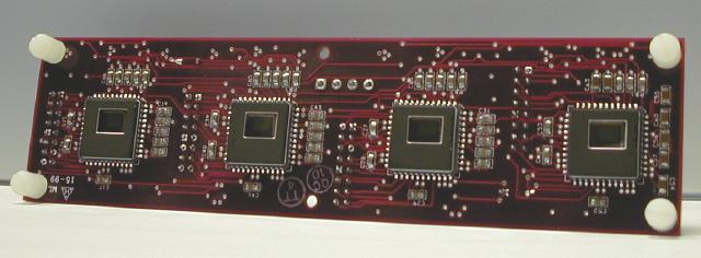
Shown below is the prototype camera tile with the lenses and lens mounts removed to show four Photobit image sensors. They are CMOS image sensors with a Bayer Mosaic color filter array and a resolution of 512x384. They have a basic auto-exposure algorithm that can be turned off (mostly), control over the gain of the red, green, and blue channels, and a few other goodies, but they have no color balancing or color correction logic.  In order to generate realistic video from these cameras, I need to implement some sort of color correction algorithm.

For this project, I investigated using polynomial models to transform from the image sensor RGB output values to device independent XYZ values. I've seen several image sensors and color processing chips that try to do this using either a direct 3x3 linear transformation or higher order polynomial models ( see [4] and [5], for example--the color correction for [5] was described at the conference but not in the paper), but I could not find a comparison of these methods, so I decided to check it out myself. It turns out that getting the experimental setup correct was tougher than checking out the different models, and I learned some useful lessons about my image sensors in specific and the color correction task in general. Finally, becuase I'm ultimately interested in making pretty pictures, I assumed some standard monitor specifications to complete the path from camera data to images ready for display on a monitor.
 

II. Methods.

Because of the number of image sensors in the planned array (possibly 100 or more), I need a relatively simple calibration method, so I decided to base my approach on the MacBeth color checker chart. Here are the steps I used:

1) Establish ground truth XYZ values for the MacBeth color checkers. Under controlled lighting, I used a spectroradiometer to measure the light reflected off the checkers on the MacBeth chart. The spectroradiometer was rigidly mounted with respect to the lights, and the color checker chart was moved to position each patch directly under the device. I multiplied the spectra by the xyz tristimulus functions to XYZ values for each checker. This was the easy part.

2) Measure RGB values for the color checkers. Under the same lighting, I replaced the photospectrometer with my camera array and repeated the measurements of the patches. In order to get accurate data, I had to account for several non-idealities of the image sensor, including the dark noise, controlling the exposure so the pixels values would not saturate, and the varying responsivities of the different colored pixels. After some trial and error, I settled on the following sequence of steps:

• Determine exposure and gain settings. I set the camera exposures and gains while looking at the white patch on the color checker. This should be the brightest spot in the image (barring specular reflections), so if those pixels were not pegged to their maximum values, the rest of the image should have been ok. The exposure settings on the imager were not directly programmable, so I had to enable the autoexposure, let it settle to an acceptable setting, then lock the exposure settings. At this point none of the pixels seemed to be saturated, but because of the reddish incandescent light and the higher red response of the imager, the red pixel values were much higher than either the green or blue ones. It is important to note that the exposure time is the same for all pixels regardless of the color gel over them, which means that the blue and green pixel voltages (at the photodiodes) will swing across a smaller voltage range. To compensate for that, I increased the gain of the green and blue channels. This gain is applied before the digital to analog converters on the chip, which means that although it does multiply the dark noise, the quantization noise remains the same, so the overall signal to noise ratio will be better. This whole process of setting the exposure and gain was trickier than it seems and involved many iterations to get nearly correct.
• Measure Dark Image. With the exposure and gain settings locked, I put the lens cap on and took ten dark images. These were averaged together and then subtracted from all the other images taken by the camera.
• Verify that the imager response is linear. Clearly, I only did this once, just to make sure that the output of the sensor was linear. I did this by plotting the recorded R, G, and B values of the grayscale color checkers versus their measured luminance values. The gain is indeed linear, but I discovered that, despite my best intentions, the two brightest patches were saturating.

Shown below is the relative quantum efficiencies of the red, green and blue pixels on the Photobit PB159DX. This accounts for the transmission of the color filters as well as the quantum efficiency of the photodetectors. Notice that the imager is much more sensitive to longer wavelength light.

This next plot shows the measured spectrum of the white MacBeth patch, which should be approximate the spectrum of our lighting. Notice that the light has more energy in the longer wavelengths, further compounding the problem of the red channel in the imager saturating.
 

This final plot shows the response of the red, green and blue channels to the grayscale MacBeth color checkers, after I attempted to set the exposure and color gain settings on the image sensor. The plot shows the the imager response is indeed linear until the pixels saturate. The saturation value, curiously, is not 256, but something less. From the plots, it is clear that the responses are extremely linear until the green and then blue and red channels saturate. The autoexposure had been fixed and the gain for the different color channels adjusted to give what looked like a pretty good distribution (from histogram data). Even so, I didn't get it exactly right. The good news is that only two of the grayscale values and one of the other color checkers had any saturated RGB values.

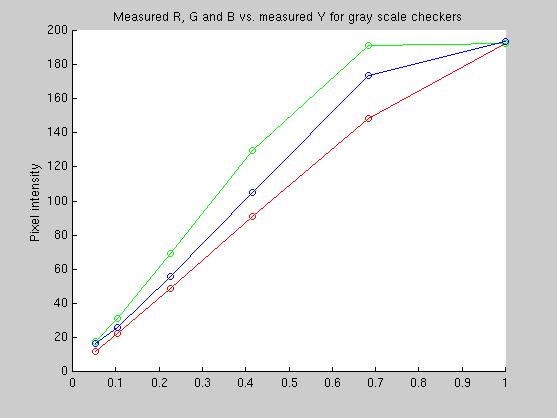
This plot
 
 

3) Calculate RGB to XYZ transformations using the different models.

• Extract patches from the images of the color checkers. For each patch, I averaged the red, green and blue pixel values of a 30x30 pixel block within the checker to get the color values used for the transformations.
• Eliminate patches that contained saturated pixels. For my setup, this turned out to be three of the twenty-four patches (the two brightest grayscale checkers, and the bright green diagonally opposite them). I simply picked a maximum allowed value and tossed any patch whose red, green or blue values exceeded the maximum. I also checked for very low values, but all were significantly over the dark noise, so this did not excluded any patches.
• Fit different models to the data.  I tried three different color correction functions, detailed in the chart below. RG represents R*G, RR is R squared, and so on.

 

Model Number	Equation	Transformatin
1	C1*[R G B]' = [X Y Z]'	C1=3x3 matrix
2	C2*[R G B RG GB BR]' = [X Y Z]'	C2=6x3 matrix
3	C2*[R G B RG GB BR RR GG BB]' = [X Y Z]'	C3=9x3 matrix

• Measure the error in XYZ and CIE-Lab space for each method.  Once I had generated the model, the next step was to compute XYZ values from the measured RGB values and compare them to the ground truth established with the spectroradiometer. In order to fairly evaluate the models, it is important to measure the error against colors that were not used to generate the coefficients for the transforms. I decided to measure two sets of errors for each model. The first was the mean squared distance error in CIE-XYZ and CIE-Lab space between XYZ values computed from the reference color checker RGB values and the measured XYZ values for the checkers. The second set measures the same errors for patches not included in the calibration set. I did not want to take any more measurements, but did want to make the fit for each model as good as possible, so I measured this error by looping through the checker chart, excluding one patch from the set used to fit the data to the model, then measuring the error of the computed XYZ value given the model and the actual value for the omitted patch. The mean squared error over the patches was generated in both CIE-XYZ and CIE-Lab space.

• Basic Bayer Mosaic Interpolation.  This is a single chip color image sensor with a Bayer Mosaic, so at each pixel it reports only one off red, green or blue. To fill in the missing data in the camera images, I just copied missing color information from the neighboring pixels. I plan to implement a more sophisticated algorithm soon. Better solutions would have been linear interpolation or an algorithm that accounts for image gradients when interpolating.
• Color Correction. I used the transformations above to correct the color in the images, according to the equations in the table above. This created images whose XYZ values should closely approximate the actual XYZ values of the scene.
• White Point Correction. The raw image data is heavily influenced by the scene lighting. The lights used for the measurements were very red, and that was reflected (no pun intended) in the recorded images. In real life, because the color constancy property of the human visual system, this reddish tint is not obvious, but when the image is displayed on a monitor under different illumination, it looks noticably red. I corrected for this by transforming from XYZ into CIE-Lab using the measured white point of the white MacBeth checker, then transforming from CIE-Lab back to XYZ using the monitor's white point.
• Device-independent XYZ to monitor dependent RGB. Rather than calibrate my monitor, I decided to use the values from the ITU-R Recommendation BT. 709, as reproduced in Charles Poynton's Colour FAQ. I figured that monitor calibration mismatch is probably a small error compared to the color correction error, but I have no guarantee that this is true. I did no gamut correction except for clipping values that were negative.
• Gamma Correction.  Finally, I implemented gamma correction assuming a monitor gamma of 2.2. This meant raising all of the pixel values to the (1/2.2) power. This is just an approximation of the standard, but the results looked ok.

The color matches for all three transformations matched pretty well. The table below lists the error to the data in the fit as well as the error to data not included in the fitting data.
 

	Colors used in fit		Colors not used in fit
Model	MSE, CIE-XYZ	MSE, CIE-Lab	MSE, CIE-XYZ	MSE, CIE-XYZ
Model 1 (RGB)	9.08e-4	52.7	1.44e-3	75.5
Model 2 (R G B RG GB BR)	4.88e-4	26.9	1.07e-3	50.8
Model 3 (nine terms...)	3.49e-4	23.7	1.55e-3	89.7

I see two lessons to be learned here. First, although the six term model is significantly better than the three term one for both colors in and out of the set used to make the fit, the improvement of Model 3 (second order, nine terms) over Model 2 (second order, six terms) is marginal for the data in the training set. More importantly, for data not used in the training set, the performance of the third model is actually worse than either of the other two models. This shows the danger of fitting with high order (even two...) polynomial models--they can be made to approximate the data used to generate them well, but for values outside that set, they can produce dramatically bad results. Thus, although Model 3 fits the colors used to create it well, it does that at the expense of the colors outside that set. Model 2 (R G B RG GB BR) is to be the best overall of the three that I tried.

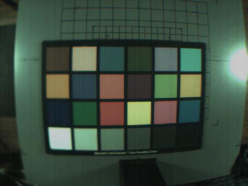
Ok, time for some pictures! First, here's one of the MacBeth color checker images, color corrected and processed for display on a generic monitor. The colors in these pictures look pretty good to me, but there are artifacts due to the simple Bayer interpolation (the wierd fringes on the checkers, for example), and incorrect gain and exposure settings (areas that saturated, like the reflection of the light and the white MacBeth checker, transform to wierd colors).

Model 1, 3x3 matrix multiply, [R G B]

Model 2, 6x3 matrix multiply, [R G B  RG  GB  BR]

Model 3, 9x3 matrix multiply, [R G B  RG  GB  BR  RR  GG  BB]

To my eyes, these three images are virtually identical, so I'll probably stick with the 3x3 first order transformation because it is the fastest and gives pretty good results. One very important caveat, though, is that the picture, which is mostly of a MacBeth color checker chart, is being transformed with matrices generated using all the colors in the chart. Model 3 is probably doing better than it deserves because as I've shown, it's less accurate when reproducing colors that were not in the model fitting dataset. Just for kicks, I took a picture of a set of random objects. Here are the color corrected results. But first, here's a telling picture to show the power of human color constancy. Here's the image above (Model 1, if you're interested), without the whitePoint adjustment in CIE-Lab space. I was looking at something very like this when I made these images, and the white and gray patches looked white and gray to me, not brown.
 

Here is the image of some random lab items.

Model 1

Model 2

Model 3

IV. Conclusions. I drew the following conclusions from this effort:

• Simple low-order models are good. Model2, the 6x3 transform from [R G B  RG  GB  BR] to [X Y Z], matched best for all data according to the XYZ and CIE-Lab error measures, but the 3x3 linear Model 1 also performed well.
• Models with too many variables are dangerous. Model3, which transforms [R G B RG  GB  BR  RR GG BB] to [X Y Z], actually performed worse than any of the other models, even though it was a better match to the data used to make the fit. Beware!
• Visually, I can't tell the difference between any of these models, and so I'll probably use the 3x3 matrix for my work because it's the simplest.
• Managing exposures, gains, and light sources for imaging is tricky business! For the case of these imagers, carefully setting the exposure and color gain settings was absolutely necessary to get reasonable data for color correction.
• This white point adaption stuff is for real. When I tried to display images on the screen without doing an adjustment using the CIE-Lab space, the images have a reddish brown tint. With the white point adaption adjustment, the images looked great. The lesson here is to make sure I know my illumination when I use these imagers.

I think a good area for work next year would be to compare these models to a tetrahedral interpolation scheme like the one used by FengXiao in his 1999 project [6]. Something interesting for me to pursue would be using the data for the relative quantum efficiencies of the different colored pixels for the image sensor to generate synthetic RGB values from different spectra. This could be used to compare the calculated RGB response with the actual imager response as well as to generate data for schemes that require a lot of samples, like the tetrahedral interpolation sheme. Unfortunately, I forgot to record the gain settings for my data, so doing this experiment will require deducing the gains or acquiring another set of images.

V. References.

[1] Adams, J. et al. "Color Processing in Digital Cameras" IEEE Micro IEEE, Nov.-Dec. 1998. vol. 18, no. 6, p.20-30.

[2] Sharma, Gaurav, and Trussell, H. Joel. "Digital Color Imaging" IEEE Transactions on Image Processing, July 1997, vol. 6, no. 7, p.901-932.

[3] Poynton, Charles. "Colour FAQ"  http://vera.inforamp.net/~poynton/ColorFAQ.html

[4] Loinaz, M. et al. "A 200 mW 3.3 V CMOS color camera IC producing 352*288 24b video at 30 frames/s" 1998 IEEE International Solid-State Circuits Conference. Digest of Technical Papers. ISSCC. Held: San Francisco, CA, USA 5-7 Feb. 1998.  p. 168-9

[5] Doswald, Daniel. "A MegaPixel Real-Time CMOS Image Processor" 2000 IEEE International Solid-State Circuits Conference. Digest of Technical Papers. ISSCC. Held: San Francisco, CA, USA Feb. 1998.

[6] Xiao, Feng and Deng, Suiqiang. "Mini Color Management System", http://www-ise.Stanford.EDU/class/psych221/99/fxiao/
 

VI. Appendix.

The code for this project is in the following files. This is every single function I wrote, some that I'm embarrased to have online-- if you want them all plus data, grab the tar file at the end.

 calibrate.m   This is the top level code. Start here.
 bayerInterp.m  Code for simple Bayer Mosaic interpolation (this is the embarassing one).
 bayerSeparate.m Code to separate a Bayer image into three color planes.
 grabEachPatch.m  Code for grabbing RGB checker values from input images, subtracts dark current.
 Model2.m     Computes the transformation matrix for Model 2.
 Model2Rgb.m  Generates [R G B RG GB BR] image for Model 2.
 Model3.m Computes the transformation matrix for Model 3.
 Model3Rgb.m   Generates [R G B RG GB BR RR GG BB] image for Model 3.
 Rgb2XyzFirstOrder.m  Transforms RGB image to XYZ image using Model 1.
 Rgb2XyzModel2.m   Transforms RGB image to XYZ image using Model 2.
 Rgb2XyzModel3.m   Transforms RGB image to XYZ image using Model 3.
 TransImg1.m  Transforms RGB input image to monitor XYZ using Model 1 & Rec 709.
 TransImg2.m   Transforms RGB input image to monitor XYZ using Model 2 & Rec 709.
 TransImg3.m   Transforms RGB input image to monitor XYZ using Model 3 & Rec 709.
 fakePhotobit.m  Generates the Photobit spectral response curves.
 myLab2Xyz     My own version of lab2xyz, I had troubles with the toolbox version.

Data and full code:

 t2mbSpecIndiv.mat  Data from the spectroradiometer for the MacBeth color checkers. Included variables are mbWave and mbSpec.

 CodeTar.gz  All the code and input data files so you can run this experiment yourself. Be sure to add the main code directory to your matlab path.