Color Correction Project: PART II

By Firas Hamze

(Part I- Calibration and correction using digital camera here.)

Color Calibration Experiments with the HP Scanjet Scanner:

The Scanner Imaging Process:

The scanner produces digital images in a similar way that a digital camera does. A illuminating light is shone onto an object with a characteristic reflectance profile (different quantities at different wavelengths are bounced back.) A mosiac of sensors recieve the reflected light and respond linearly to the intensity. Scanners, however, perform a gamma-correction process whose purpose is to straighten the nonlinear relation between CRT intensities and frame buffer values that would otherwise warp the color appearance.

Calibration:

A scanned image, however, may not closely resemble the original when displayed on a monitor. Color-calibration systems attempt to resolve these discrepancies. Percieved colors are often described in terms of their xyz values, the relative quantities of given primary lights used by a person to match a color stimulus. Thus, perceptual correspondence between the original image and the scanned, displayed image is achieved if the xyz values are concurrent. In the experiments described here, we attempt to find an agreement between the original image xyz values and the xyz values of the scanned image.

Experimental Procedure:

Scanning the Input Data:

The first step was to scan a color source; we used the Macbeth Color Checker, displayed in Figure 1.

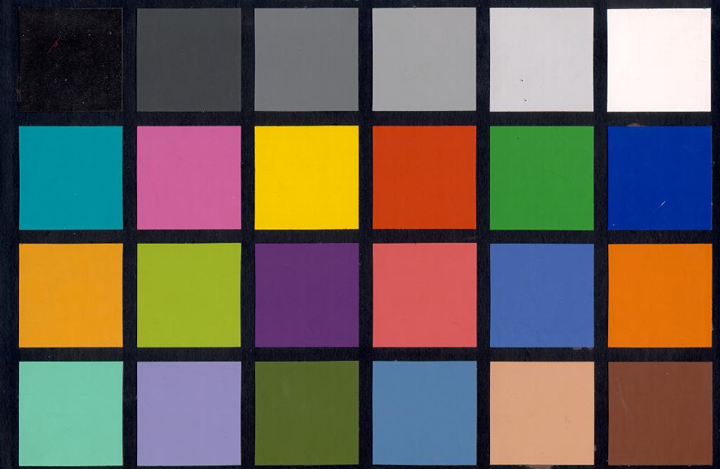
Figure 1: The Macbeth Color Checker used to get color data.

Extract patch reflectance values and compute xyz:

In order to obtain its xyz values, the spectral reflectances of the surfaces must be known. This was done as follows: the white patch of the checker was assumed to represent the spectral distribution of the tungsten light source. This light was divided away at each wavelength (since the reflection is linear) to leave us with the reflectances. This is shown pictorially in Figure 2. The xyz relation is the xyz color matching function multiplied by the spectral radiance of the surface under the scanner light.

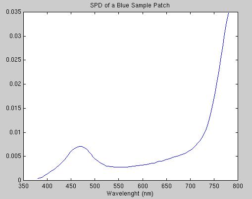
Figure 2(a): The spectral power distribution of the blue patch shown in 2(d) subject to the light shown in 2(b).

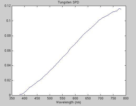
Figure 2(b): Spectral power distribution of the tungsten light source used to get the xyz data of the patches.

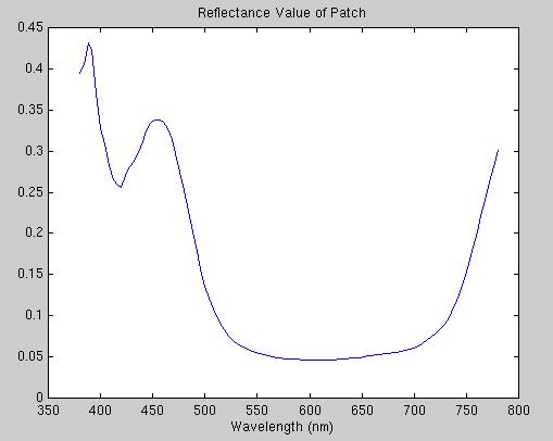
Figure 2(c): Reflectance profile of the blue patch shown in (d). Figure 2(d)

We ran into several practical difficulies in obtaining the spectrum of the scanner light, so the assumption was made that standard D65 white light is used. The spectrum of this light is shown in Figure 3.

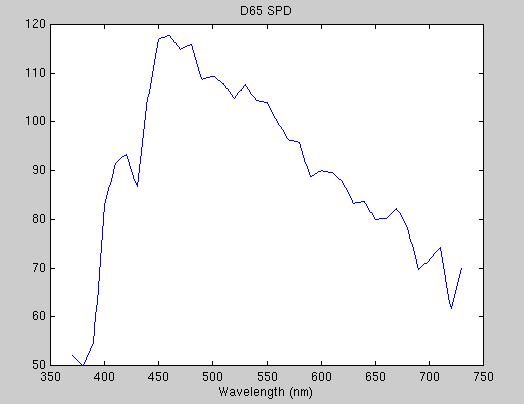
Figure 3: Power distribution of white light.

Compensate for gamma correction in the scanner:

The scanner, however, performed gamma-correction on the light, so that the presumably linear reponse of the sensors was skewed. This effect is shown in Figure 4, where the mean RGB values for the gray test patches is plotted against the intensity of the patches as measured by the luminance component of the spectroradiometer with the light source removed. The gamma factor was computed by finding the parameter that made the logarithmic relation derived from the gamma function be the best fitting line to the data (see the code for details.)

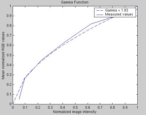
Figure 4: The gamma function. Solid line is the plot of measured data, the dotted line is that of our best-fitting value of gamma = 1.83.

Fit to first- and second-order linear models:

We searched for a relation between the RGB and the xyz values using both a first- and second-order model described in the section on camera calibration. Each test patch's RGB values were normalized to the range [0,1] and transformed by the inverse of the gamma relation described above. Thus, we obtain the RGB values that for the given light intensity would have resulted. We now have a linear relation between the intensity and the value of the RGB. The patch xyz values are, as stated earlier, calculated from the radiometric data and the presumed light source.

It remains to compute a matrix that transforms from the RGB to the xyz values. 12 of the 24 Macbeth color patches were used as data to determine the matrix, and the remaining 12 were used to test it. The data patches were gamma-corrected and the matrix solving the relation A(rgb) = (xyz) was solved using the known xyz values, and the matrices from the 2 methods were applied to the test patches and the xyz values were compared.

Conclusion:

Unlike those relatively successful results of the camera calibration, the scanner did not seem to be tractable by our model. The actual xyz values of the test patches are shown below:

xyz =

    0.3883    0.1806    0.3319    0.1119    0.3511    0.4683    0.1225    0.4025    0.2153    0.1132    0.2798    0.3659
    0.3134    0.1712    0.2266    0.0862    0.4508    0.4387    0.1066    0.3780    0.2274    0.1465    0.2662    0.4929
    0.0638    0.4593    0.1671    0.1950    0.1272    0.0908    0.0669    0.2788    0.4254    0.0776    0.4891    0.5380

and the first-order model-predicted values are:
xyz =

    0.5552    1.4108    0.6246    0.3804    0.3162    1.3409    0.7482    0.7298    0.0636   -0.4542    1.4210    0.3061
    0.4389    0.4101    0.4300    0.2138    0.2589    0.7208    0.3189    0.6474    0.0668    0.2721    0.4604    0.5073
    0.4515    0.0772    0.5551    0.1115    0.2701    0.8538    0.0781    0.7438    0.0875    0.2735    0.2602    0.4493

and second-order values are:
xyz =

    0.8229    0.3366    0.9697    0.7439    0.5614    2.2723    0.8255     1.0459    0.0892   -0.8363    0.7409    0.0236
    0.5879    0.1557    0.2040    0.4472    0.4212   -0.4086   0.3161     0.5884    0.0907    2.2968    0.4936    1.7329
    0.5397    0.3945    0.2260    0.2338    0.3858   -0.7411   0.1060     0.5722    0.1252    2.6730    0.6339    1.8827

The mean-square error in prediction for the first order model was:

mse = 0.1817
and
mse = 0.6516

for the second-order model.

There are several reasons why this could occurr. Most obviously, yet most probably, the error was caused by the fact that the scanner light source was not D65. This would skew the actual xyz values. Also, the measured gamma value (1.82) was not the same as the gamma specified in the scanner program (2.23.) We attempted to experiment with the effect of varying gamma on the xyz values; the change never made the results substantially more accurate.

Appendix:

Code to compute the mean RGB values of a color patch: getRGB.m
Computes the value of gamma and plots it: plotGamma.m
Performs the inverse gamma correction on the rgb: gammaCorrect.m
Gives the linear transformation matrix(1st or 2nd order): train.m
Runs the transformation over test data: testt.m
Perform 1st order fitting: o1fit.m
Perform 2nd order fitting: o2fit.m

References:

See Part 1 on camera calibration.