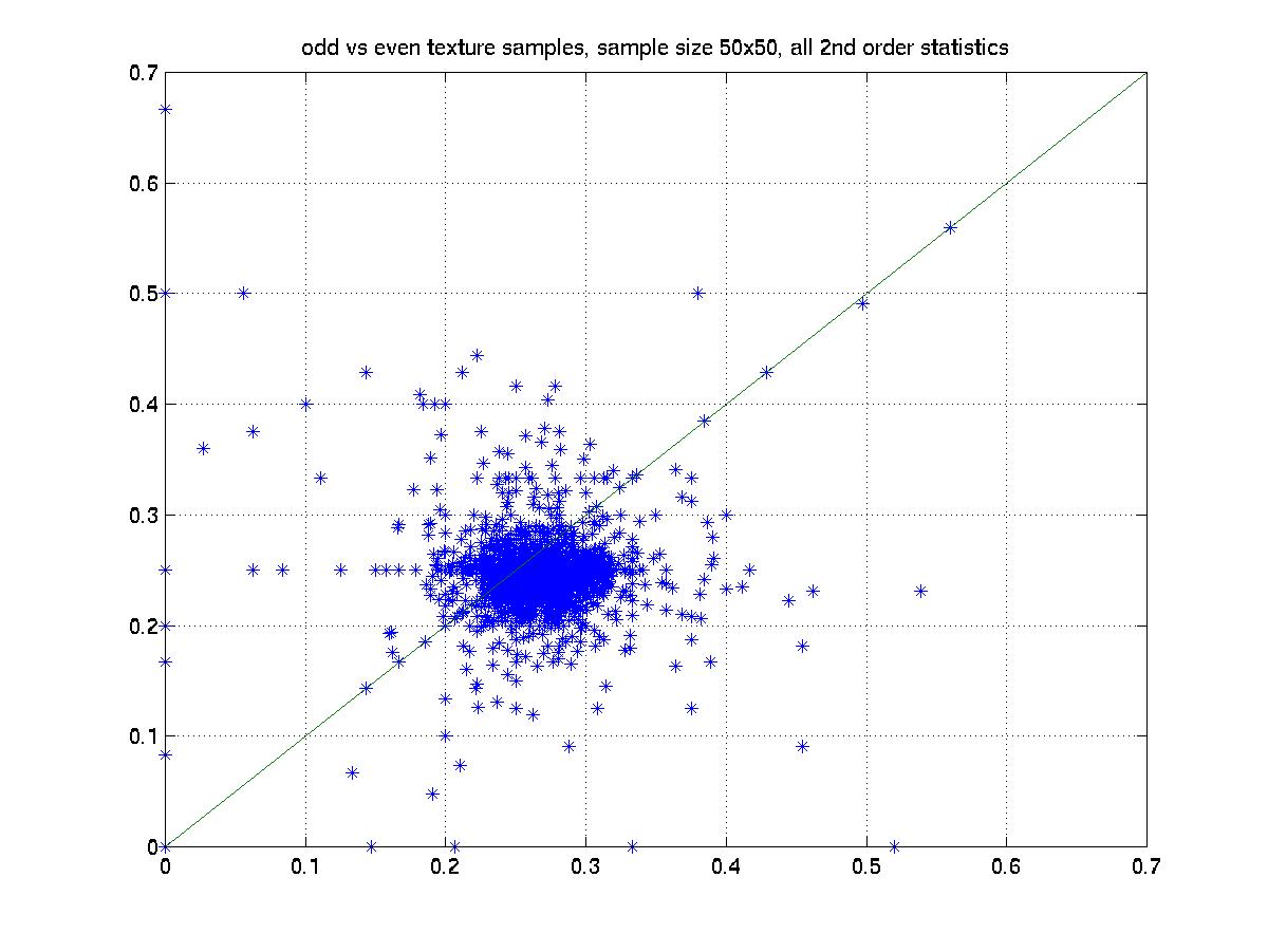
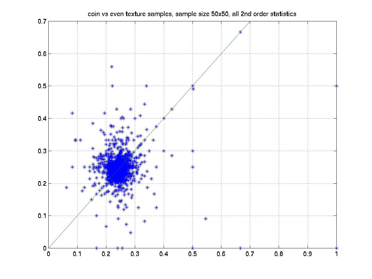
Although Julesz's Conjecture has been proved wrong by himself through the odd and even texture images mentioned before, Yellott didn't agree with his result completely. The identical second-order statistics of the odd and even textures are the result the odd and even stochastic image generating process, not the images themselves. We can easily generate the odd, even and coin-flip images according to Julesz's algorithm and calculate their second and third order statistics.

Even Vs Odd Textures
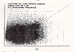
Second-order statistics	Third-order statistics

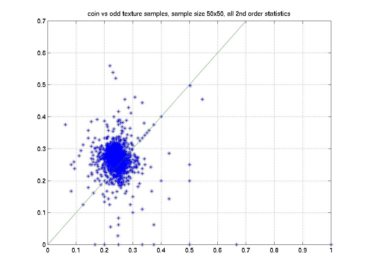
Coin-flip Vs Odd Textures
Second-order statistics	Third-order statistics

Even Vs Coin-flip Textures
Second-order statistics	Third-order statistics

The X axis is the statistics of one texture and the Y axis is the other texture. Hence if the corresponding statistics are the same, then all the points should fall on the X=Y line, which is drawn as a reference.

Apparently the above results show that neither second nor third order statistics of these texture images are the same.

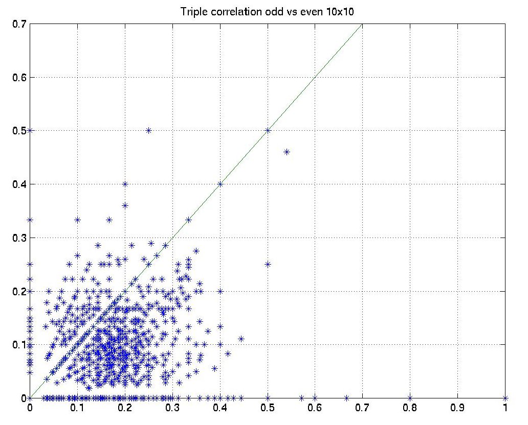
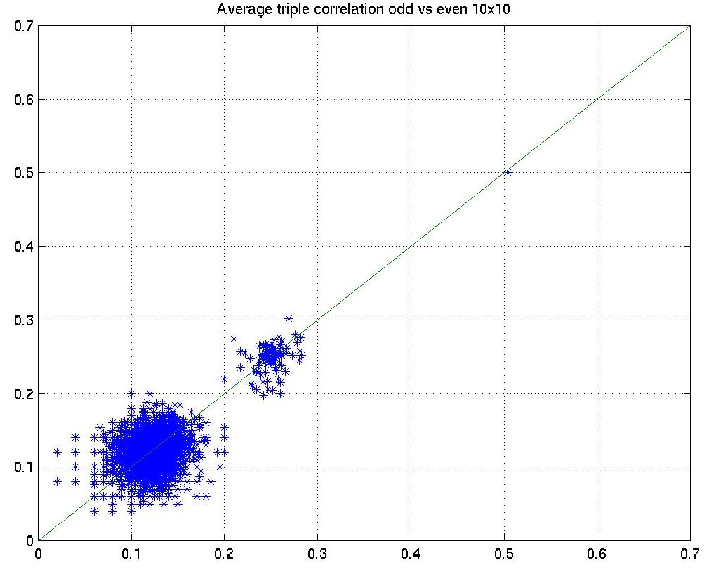
Actually it varies a lot. To avoid the comples proof of the identical second-order ensemble statistics, we use a little experiment to show it. Since the calculation of triple correlation for large images is extermely time-consuming, we adopted much smaller 10x10 odd and even texture pairs. We generated 100 pairs and calculated the second-order statistics. Both the scatterplot and histogram show that the averages are quite closed to each other.

Triple correlations Odd vs. Even
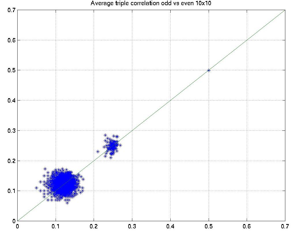A single texture	Average of 50 textures	Average of 100 textures

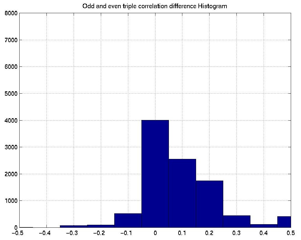
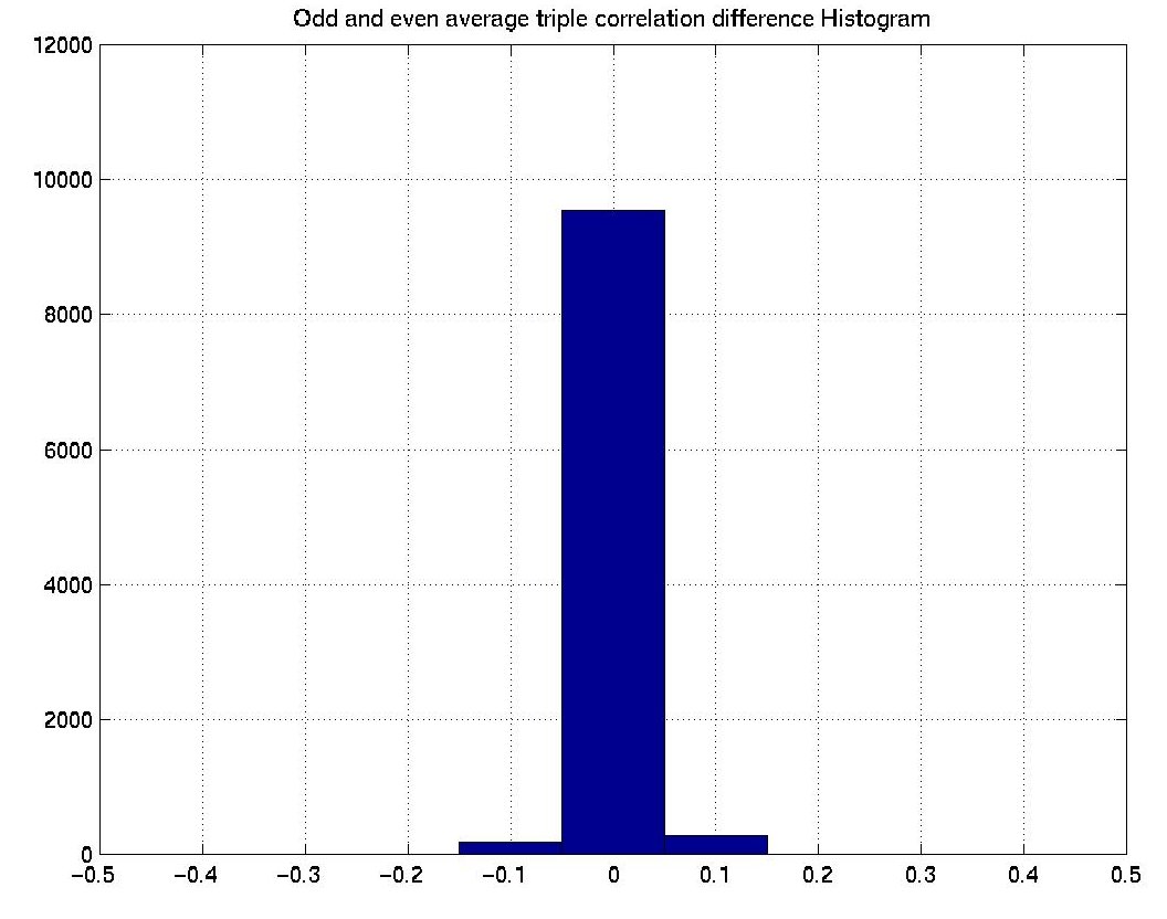
Triple correlations difference histogram Odd vs. Even
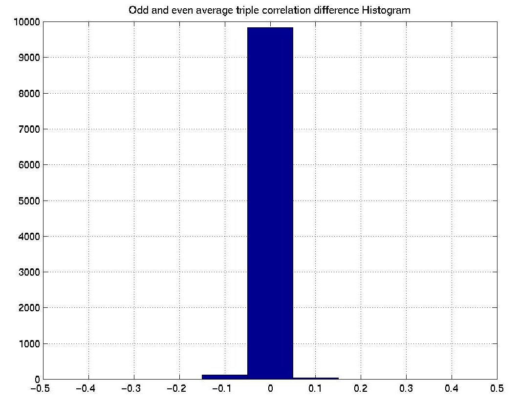A single texture	Average of 50 textures	Average of 100 textures

Similar results can also be acquired if the size of these odd and even texture images are infinite.

However in practice, all images must be finite. Yellott thought Julesz's arguments based on identical second-order ensemble statistics isn't quite right.

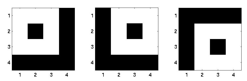
In his paper, Yellott proposed the Triple Correlation Uniqueness Theorem , which is very similar to Julesz's Conjecture and applicable to finite images. He also provided counter examples to Julesz's Conjecture with deterministic identical second-order statistics but is spontaneously discriminable.

If f is an image function with bounded support, and another image g has the same triple correlation function as that of f, then g(x,y)=f(x+a,y+b) for some pair of constants a and b.

A complete proof is too long to be necessary here. We briefly describe the steps of the proof and choose a 1-D image for simplicity.

Suppose two images f(x),g(x) have the same triple correlation function, the their Fourier tranforms F(u),G(u)satisfy the relationship:

F(u)F(v)F(-u-v)=G(u)G(v)G(-u-v)

If u=v=0, then F(0)=G(0)

Without loss of generality, choose F(0)=G(0)=1, then treat f(x), g(x) as probability density function and F(u), G(u) as characteristic functions.

Choose v=-u, then | F(u) |=| G(u) |;

Consider the phase:

phase(G(u))+phase(G(v))-phase(G(u+v))=phase(F(u))+phase(F(v))-phase(F(u+v))

Let D(u)=phase(G(u))-phase(F(u))

D(u+v)=D(u)+D(v)

By the properties of characteristic functions, only solution for D(u) is D(u)=bu=2*pi*c*u

phase(G(u))=phase(F(u))+2*pi*c*u

G(u)=exp(i*2*pi*c*u)*F(u)

g(x)=f(x+c)

One original and two translated images

We have tested the examples in the above. The triple correlations are all the same.

• Reconstruction from finite Images

  Since the uniqueness has been proved, any image should be able to reconstruct from its triple correlation, up to a translated version.

  Basic ideas: (still 1-D image)

  The Fourier transform of triple correlation tr(x,y), TR(u,v):

  TR(u,v)=F(u)F(v)F(-u-v)

  |F(u)|=(TR(u,0)/TR(0,0)^(1/3))^(1/2)

  phase(F(u+v))=phase(F(u))+phase(F(v))-phase(TR(u,v))

  The magnitude of Fourier transform F(u) of image f(x) is easy to determine. The phase is more difficult. It can be found by some recursive algorithm. When the F(u) is determined, the f(x) can be easily reconstructed.

Basic concepts:

For p(x,y) and p(-x,-y), they have the same power spectrum and autocorrelation function but they will look different if they are not symmetric.

People may argue that some people might want to treat rotated images as the same. Hence Yellott proposed that we can distribute the micropattern by the convolution with delta functions so that they might "look" different.

For p(x,y)*q(x,y) and p(x,y)*q(-x,-y), they still have the same power spectrum and autocorrelation functions. Since we are now considering only black and white images. We must be careful that the delta functions won't make the micropattern overlap.

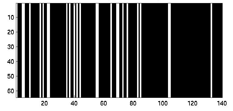
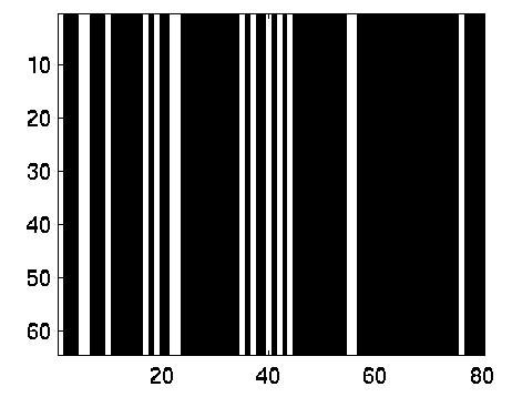
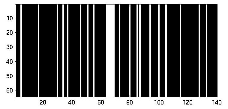
An 1-D example was provided by Yellott:

p(x)=sum(delta(x-4*n*n))     n=0:4

p(x)=sum(delta(x-(4*n*n+n+1)))     n=0:4

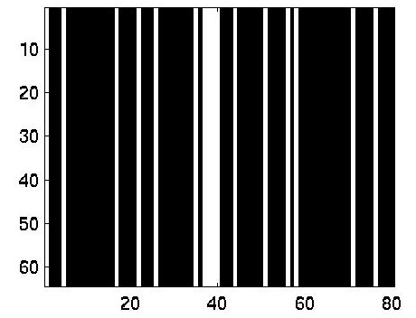n=4	n=3

The 2-D examples: Replicates of micropattern, letter T

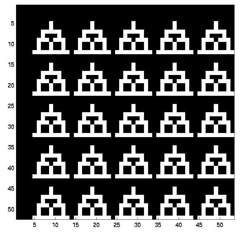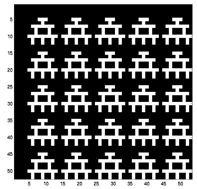All the second-order statistics of the counter example images have been checked to be the same.