WEB PHOTO EVALUATIONS: NOISE ANALYSIS

Introduction

In this report, we summarized our investigations and evaluations of noise for the digital images processed by several photographic companies. First, we described the setup of the experiment and explained the purposes of preliminary tests. Second, we analyzed the noise reduction processes by calculating the mean and standard deviation (STD) of each Red, Green, and Blue (R, G, and B) component of the image. Third, we studied the distributions of noise across the entire images and analyzed the one-dimensional signal waveforms. Fourth, we computed the Signal to Noise Ratio (SNR) based on the mean and STD of the corresponding images. Finally, we concluded our investigations by comparing these companies according to the performance of noise elimination processes.

Experimental Setup

In this section, we outlined the setup of our experiment in order to analyze the noise reduction processes for each photographic manufacturing company. We also demonstrated several preliminary evaluations to confirm the reliability and credibility of the photo scanner. The goal of these preliminary tests is to make sure that the scanner is capable of capturing high frequency signals and producing insignificant random noise comparing with the noise that is added to the images. Moreover, the Matlab programs are attached at the appendix section of this report.

I. Experiment Design

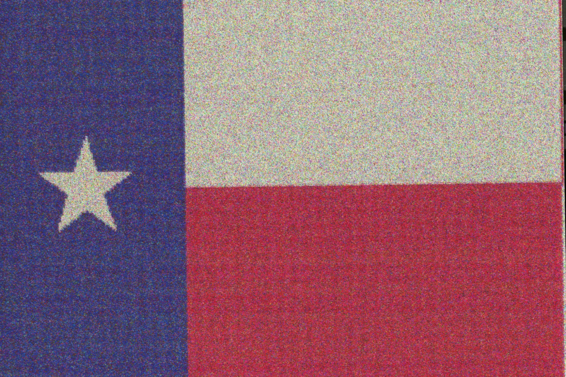
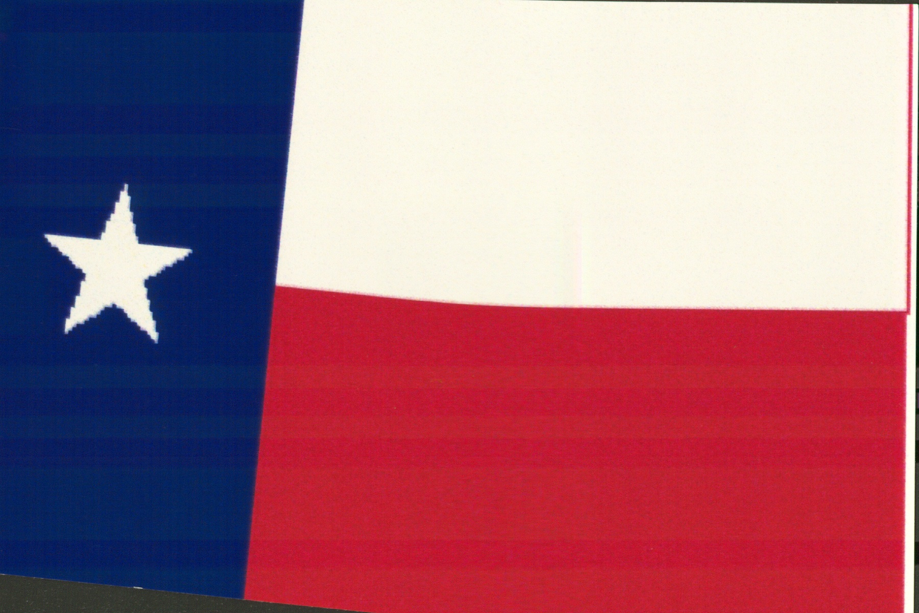
We designed our experiment by creating six Texas flag images with different Gaussian noises. Each added Gaussian noise has zero mean with variance varying from 0 to 0.5. We first uploaded these pictures to the web and sent each company the same set of pictures. After each company returned these pictures, we then scanned these pictures back into the photo scanner and converted these images into digital format. Finally, we analyzed the images by comparing the statistical characteristics and signal properties according to each R, G, and B components. Figure 1 shows the pictures that we designed.

Figure1: Designed Texas Flag Images

Pictures

Variances

0.02

0.05

0.1

0.2

0.5

II. Preliminary Tests

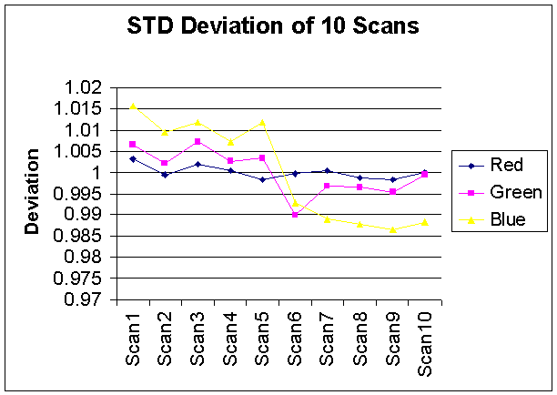
Before we implemented our analyses, we first needed to evaluate the reliability of the HP photo scanner and the random noise that is generated by the scanning processes. In order to evaluate these parameters, we scanned the same image ten times and computed the means and STD of these pictures. Our results showed that the data we collected only deviates by ± 0.5 %. Figure 2 and 3 show the deviation of the mean and STD of these ten scans.

Figure 2: Mean Deviation of 10 Scans

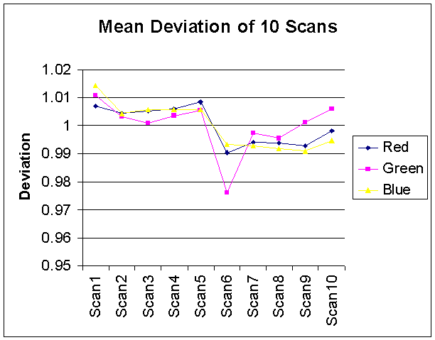
Figure 3: STD Deviation of 10 Scans

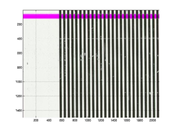
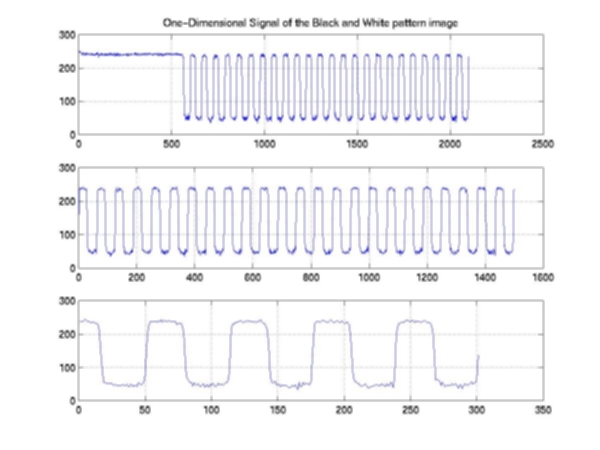
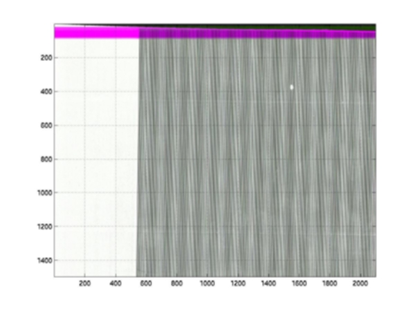
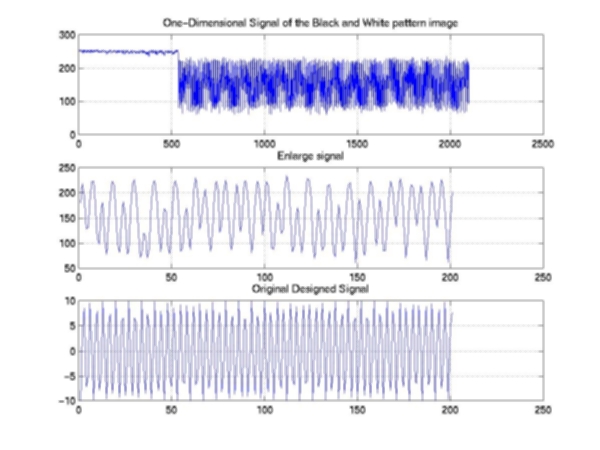
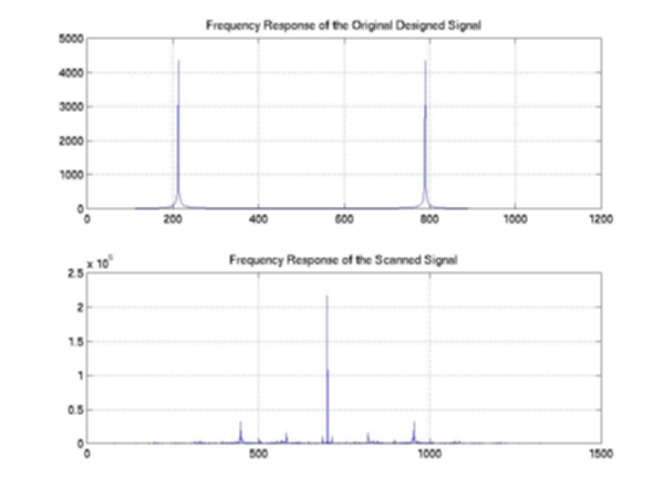
Our second step is to investigate the scanner’s capability to capture the high frequency response of the image. We created a sample image with alternating black and white lines by generating a sinusoidal signal of a constant carrier frequency. We then printed and scanned the image into the scanner to compare the captured signal with the one that we created. Figure 4 shows the black and white line pattern with 80 Hz central frequencies and Figure 5 shows the corresponding one-dimensional signal. In order to investigate the high frequency response of the scanner, we designed the same black and white pattern with 288 Hz carrier frequencies (Figure6 & 7). Our results showed that the scanner does a good job on capturing these high frequency signals. Furthermore, we also computed the one-dimensional Fast Fourier Transform for both the designed and captured signals (Figure 8). In the frequency domain, we can clearly observe the peaks at the corresponding carrier frequency. In other words, the noise that we observed in the captured signal is more likely due to the printing processing, but not to the scanning processing. As a result, based on both preliminary tests, we can certainly confirm that the scanner can produce reliable digital images and the random noise that is generated by the scanning processing is relative small comparing to the noise that we added to the images.

Figure 4: Black & White Line Pattern with 80 Hz Carrier Frequencies

Figure 5: One-Dimensional Signal of the Black & White Pattern

Figure 6: Black & White Line Pattern with 288 Hz Carrier Frequencies

Figure 7: One-Dimensional Signal of the Black & White Pattern

Figure 8: Frequency Response of the Signals

Data Analysis and Results

In this section, we will summarize our noise analyses by computing the mean and STD of each R, G, B component of the images. By comparing the mean and STD of the images that processed by different companies, we can evaluate the noise reduction processing. We also estimated Large Area and One-Dimensional SNR and investigated the variations of signals across the entire images. Furthermore, we ranked each company according to each evaluation function that we developed.

For our conveniences, we represented the name of each company by their abbreviations and numbered each image according to the corresponding noise variances. Table 1 provides the complete list of our notations.

Table 1: Notations and Abbreviations of the Images

Companies	Abbreviations	Image Number	Meaning
Original Designed Images	Org	41	Image with no noise
ShutterFly	Fly	42	Variance = 0.02
Ofoto	Ofoto	43	Variance = 0.05
PhotoNet	Net	44	Variance = 0.1
PhotoAccess	Access	45	Variance = 0.2
		46	Variance = 0.5

I. Mean & Standard Deviation of the Entire Images

Figure 9, 10, and 11 show the histograms of mean values for each R, G, and B component, respectively. For the original designed images, we observed that the mean decreases as the noise level increases for both R and B components. In contrast, the mean is directly proportional to the noise level for the G component of the same set of images. For the ShutterFly images, the means are lower than the original images for R and B components but higher for the G component. For PhotoNet images, the means are about the same for G and B components. In addition, the mean values of the PhotoAccess images are even greater than the ones of the original images.

Figure 9: Histogram of Average Values for Red Component

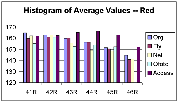
Figure 10: Histogram of Average Values for Green Component

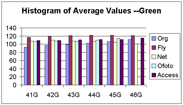
Figure 11: Histogram of Average Values for Blue Component

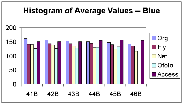
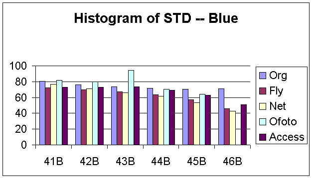
Figure 12, 13 and 14 show the histograms of the STD for each R, G, and B components. As expected, for the original images, the STDs decrease as the noise variances increase. We evaluated the noise reduction processing by studying how well could the images processed by these companies matched our designed images in term of means and STD. However, the percentages of mean and STDs decreases are relatively small for all images processed by each company. We certainly could not evaluate the noise reduction processes of these companies just based on the variations of means and STDs. Therefore, we needed to investigate the distributions of noise across the entire image by decomposing the images into a set of blocks.

Figure 12: Histogram of STD for Red Component

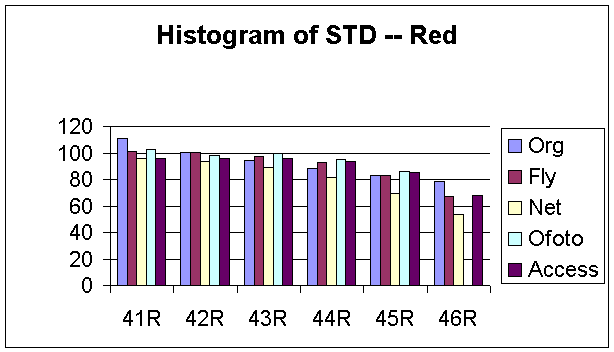
Figure 13: Histogram of STD for Green Component

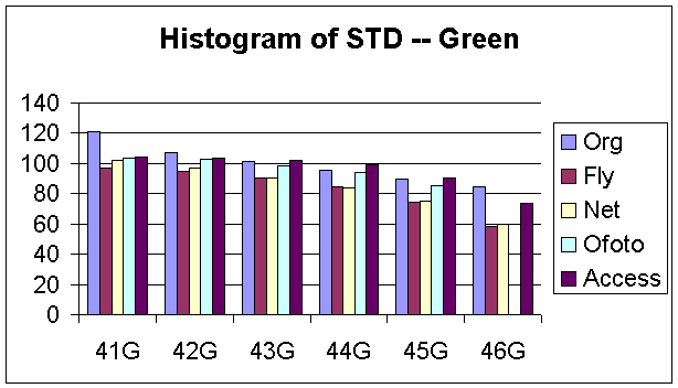
Figure 14: Histogram of STD for Blue Component

II. Mean & Standard Deviation of the Decomposed Images

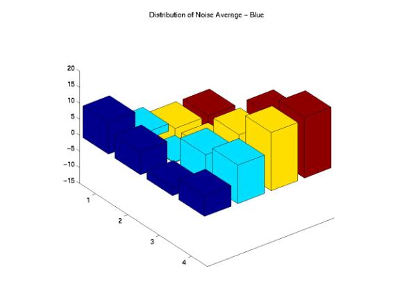
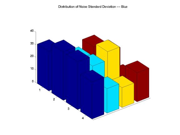
Figure 15, 16, 17, 18, and 19 are the distributions of noise average across the entire image for the B component. We certainly observed that the noises for the ShutterFly, Ofoto, and PhotoAccess images are not uniformly distributed across the image. Specifically, the processes of both PhotoAccess and Ofoto well eliminated noises in the upper corner of the images. The processes of ShutterFly actually added more noises in one region and eliminated too many noises in the other region. Additionally, the noise distributions of the images processed by PhotoNet matched perfectly with the original images.

Figure 15: Noise Average Distributions of the Original Image

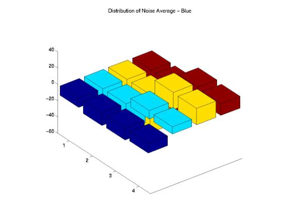
Figure 16: Noise Average Distributions of the ShutterFly Image

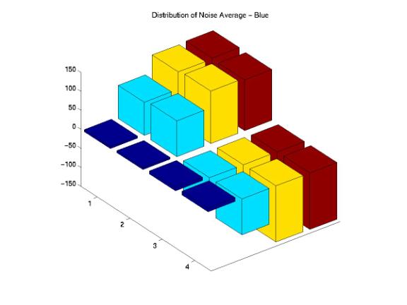
Figure 17: Noise Average Distributions of the PhotoNet Image

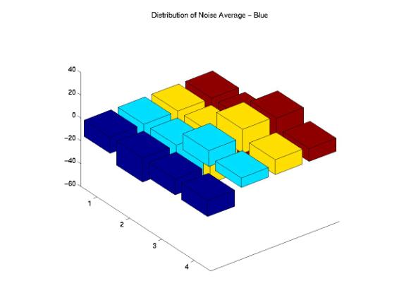
Figure 18: Noise Average Distributions of the Ofoto Image

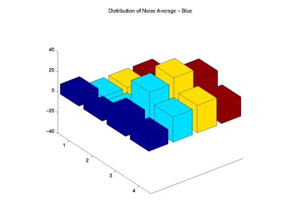
Figure 19: Noise Average Distributions of the PhotoAccess Image

On the other hand, we also investigated the distributions of noise STDs across the images and compared these distributions with the designed images. Figure 20, 21, 22, 23, and 24 show interesting results as we correlated these STD distributions with the corresponding mean distributions. The original STD is quite uniformly distributed across the image except one block at the corner of the image. Although the PhotoNet, Ofoto, and PhotoAccess distributions show different kinds of variations, the center regions of the STD distributions matched with the original distribution. The STD distribution of ShutterFly image shows little noise variations around the edges of the image and extreme high noise variations around the central region of the image.

Figure 20: Noise STD Distributions of the Original Image

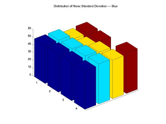
Figure 21: Noise STD Distributions of the ShutterFly Image

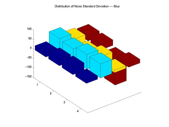
Figure 22: Noise STD Distributions of the PhotoNet Image

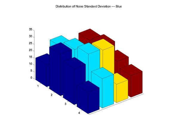
Figure 23: Noise STD Distributions of the Ofoto Image

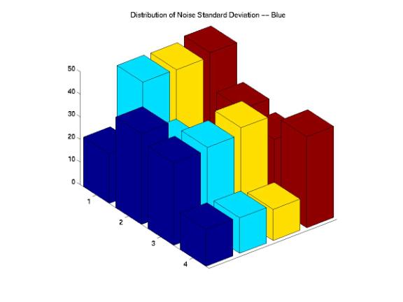
Figure 24: Noise STD Distributions of the PhotoAccess Image

III. One-Dimensional Signal Analysis

We analyzed the one-dimensional signals along the same horizontal line across the images processed by these companies. In order to investigate the distributions of the signals, we studied the sample signals along both the edge and the center of the images. Figure 25, 26, and 27 show the one-dimensional signals along the same horizontal line at the center with 0.05, 0.1, and 0.2 variances. We found a significant amount of noises that were eliminated at all noise levels. The PhotoAccess signals are relatively smoother than the signals for the other companies. Both of the edges of the ShutterFly and PhotoNet signals are blurred. As a result, the image features are either enlarged or shifted with respect to the original features. Furthermore, the signals along the edges of the images provide significant evidences to demonstrate the non-informality of the noise elimination processes (Figure 28, 29, and 30). We identified the improper rising or falling edges for both PhotoNet and Ofoto signals. These improper edges indicated that while we would not identify the shifting or blurring of the image features by the naked eyes, the features actually are not correlated with the designed images. Moreover, the PhotoNet signal with 0.1 variances is completely lost and the Ofoto signal with 0.2 variances is flat except an impulse around the location where the edge supposed to be.

Figure 25: One-Dimensional Center Signal with Variances = 0.05

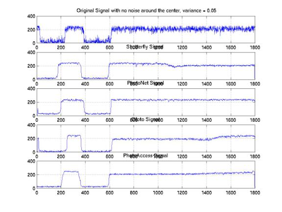
Figure 26: One-Dimensional Center Signal with Variances = 0.1

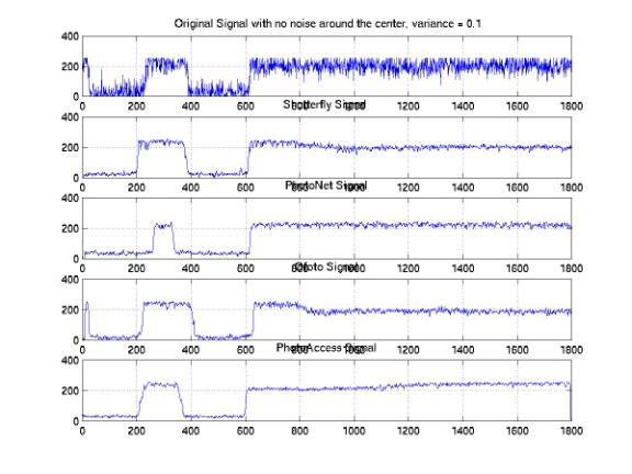
Figure 27: One-Dimensional Center Signal with Variances = 0.2

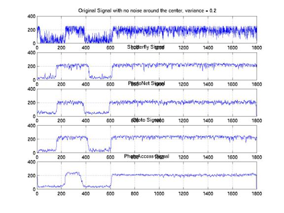
Figure 28: One-Dimensional Edge Signal with Variances = 0.05

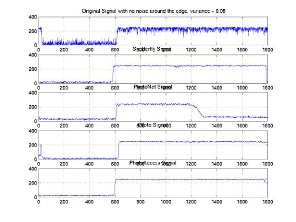
Figure 29: One-Dimensional Edge Signal with Variances = 0.1

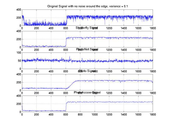
Figure 30: One-Dimensional Edge Signal with Variances = 0.2

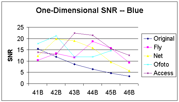
VI: One-Dimensional Signal to Noise Ratio

The one-dimensional SNR is estimated according to the following formula:

SNR = average of signal / STD of signal

Based on this formula, we expected that the one-dimensional SNR should decrease as noise increases because we designed these images by increasing noise variances. Our calculations show the same relationship in all R, G, and B components for the original designed images (Figure 31, 32 and 33). We observed that the one-dimensional SNR for the images processed by PhotoAccess is much greater than the other companies in all R, G, and B components. In addition, the one-dimensional SNR for the PhotoAccess image with 0.5 variances is even greater than the SNR for the one with no noise. These results show that the PhotoAccess imaging processing not only reduced the noise, but also raised the signal level. On the other hand, the one-dimensional SNR for the image that processed by PhotoNet first increases as the variances increase from 0 to 0.02 and then decreases as the variances increase from 0.05 to 0.5. This result indicates that PhotoNet’s noise reduction processing was capable for eliminating low level noise but failed to reduce high level noise. Additionally, the noise reduction processes for Ofoto was worst for noise with 0.05 variances since the corresponding one-dimensional SNR has lowest value as comparing with the image with the same variances.

Figure 31: One-Dimensional SNR of Red Component

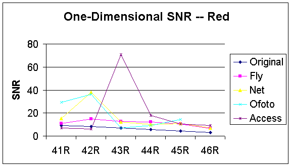
Figure 32 : One-Dimensional SNR of Green Component

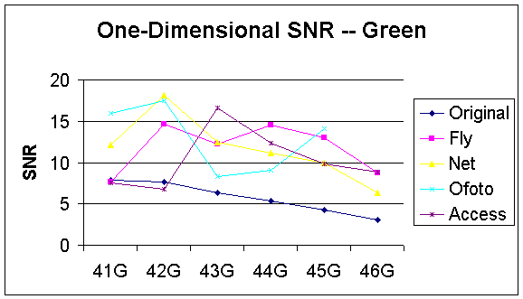
Figure 33: One-Dimensional SNR of Blue Component

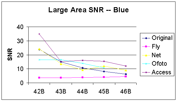
V. Large Area Signal to Noise Ratio

The International Organization For Standardizations (ISO) defined the Large Area SNR for noise measurements of digital camera in 1999 [1]. Because the noise measurement standard for digital images is not established, we modified the ISO Large Area SNR definition and redefined it according to the following formula:

Large Area SNR = maximum level * 0.18 / ( Average of the total noise * incremental gain)

· maximum level is the maximum digital level for an eight-bit system, which equals to 255

· Average of the total noise is the average of the standard deviation of “M x N” samples of the total noise.

· Incremental gain is defined to be 0.1

According to our computations, the Large Area SNR for the original designed images decreases as the noise level increases (Figure 34, 35, and 36). For all R, G, and B components, the Large Area SNR for the images processed by PhotoAccess is greater than the same images processed by other companies as the noise variances increase from 0.1 to 0.5. Although the Large Area SNR for the PhotoAccess image with 0.02 variances is less than the one for the corresponding original designed image, the noise reduction processing by PhotoAccess is much better than the other companies in general. On the other hand, the Large Area SNR for the images processed by ShutterFly is much lower in magnitude than the same set of images processed by other companies, even for the image with no noise. However, the ShutterFly Large Area SNR actually increases as noise level increases for both G and B components.

Figure 34: Large Area SNR of Red Component

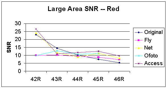
Figure 35: Large Area SNR of Blue Component

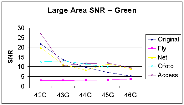
Figure 36: Large Area SNR of Blue Component

Conclusions

Based on our previous analyses, we summarized our investigations in the following list:

• Each company does a good job on eliminating the noises added to the images. In general, the images processed by PhotoAccess tend to eliminate more noises than the others.

• As the variances of the Gaussian noises increase, the means and STD of each R, G, and B component actually decrease.

• The noises across the entire images are not uniformly distributed. Some images are taken off more noises than what we added.

• The images processed by PhotoAccess, and PhotoNet both have higher one-dimensional and Large Area SNR.

References

[1] International Organization for Standardization Technical Committee 42, “ISO/TC42N 4430 Photography – Electronic still

picture cameras – Noise measurements,” Photographic and Imaging Manufacturers Association, Inc., June, 1999.

Appendix

The Original Designed Images

The Images that each company sent back to us:

Fly41.jpg Fly42.jpg Fly43.jpg

Fly44.jpg Fly45.jpg Fly46.jpg

Net41.jpg Net42.jpg Net43.jpg