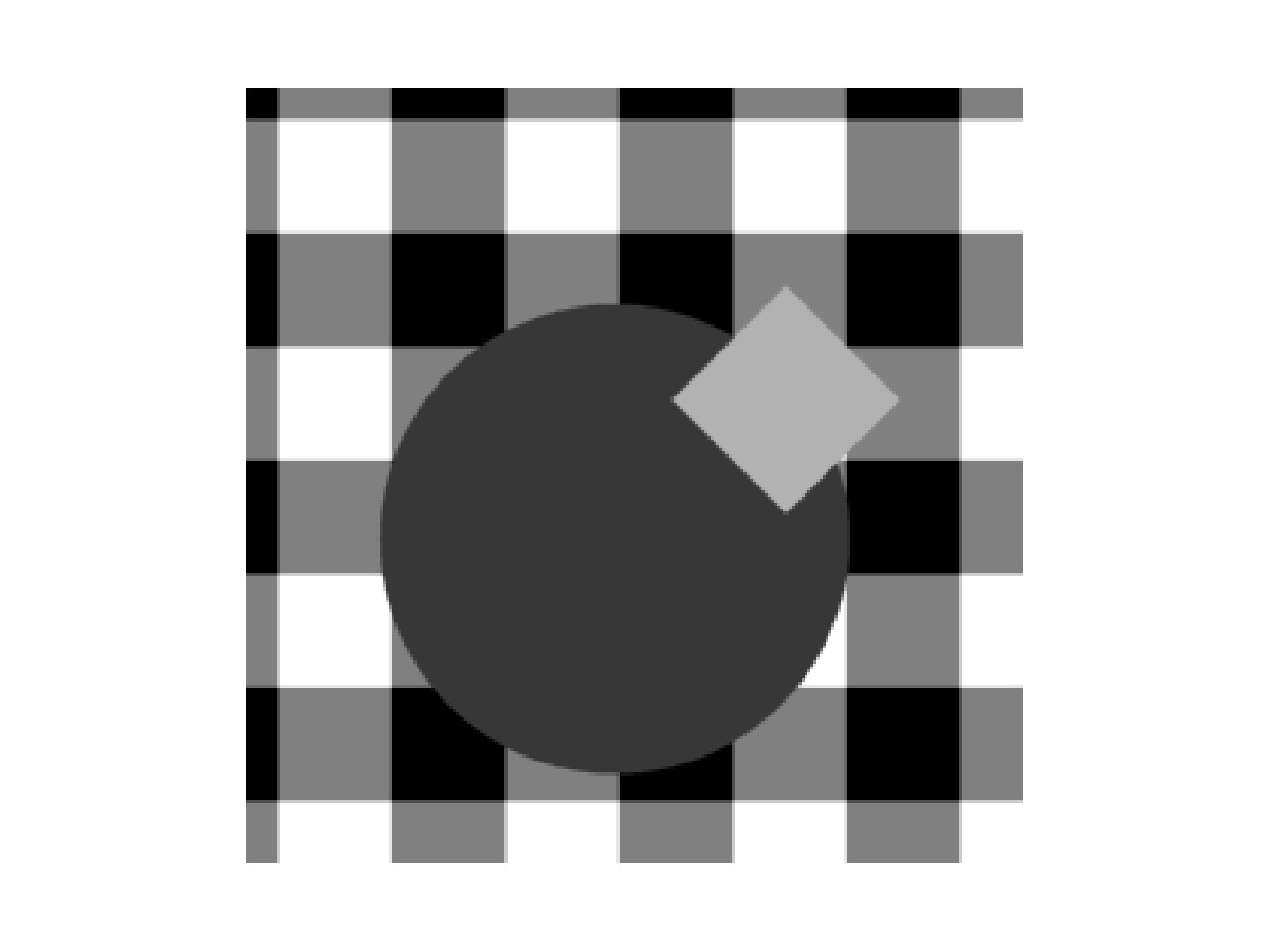
< Figure: Before zooming >
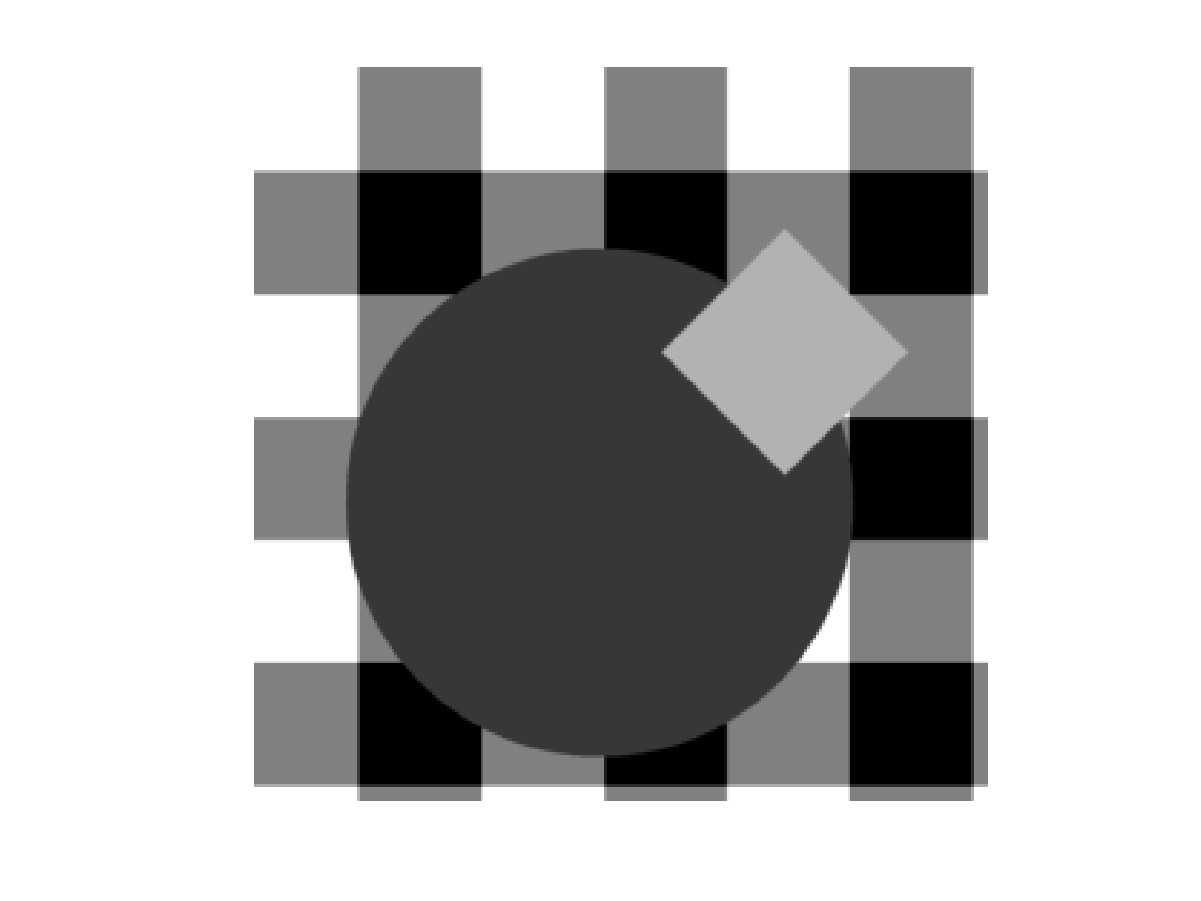
<Figure: After zooming >
The simulation environment( object
image generation ) and how the algorithm was implemented in MATLAB is described.
Also some issues regarding implementation is also listed.
First, a checkerboard pattern background was created. This checkerboard pattern was chosen to account for the fact that a background does not have uniform brightness levels. And after that, objects like square, circle, diamond were added to the image. Occlusions are also handled by the order of adding each objects.
Up to now, we have generated a scene. To simulate bluring by area integration of pixels in cameras, the scene was locally averaged and subsampled yielding an image captured by a camera. The capturing area and size was made flexible to simulate camera translation and zooming effect. Because of this sub-sampling, simulation of object motion could be achieved with sub pixel accuracy. In the image that was created for implementation of the algorithm, the subsampling ratio was 4, so that we can simulate object movement up to quarter-pixel accuracy.
Matlab codes- generation.m
| background.m | capture.m
| circle.m | ob-square.m
| square.m
< Figure: Before zooming >
<Figure: After zooming >
However, as I started coding this algorithm in MATLAB, it was a nightmare. Even though the number of operations needed for this is small, addressing was a major disaster. So, the overall complexity for this algorithm is not so low as I expected. Since objects have a random shape, it is very hard to link all the edges so that MATLAB understands the set of edge point as an object.
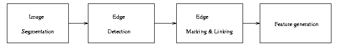
< top.m
& region.m >
< seg.m >
< marking.m & link.m
> < featuremap.m
>
This algorithm is also very well suited
for pixel level processing. Since the communication between pixels are
limited to the nearest neighbors, the communication overhead is very small.
Pixel level processing makes thing highly parallel so that it can be applied
to high speed imaging. One problem occurs when we want to extract feature
values from the edge pixels.