For the sake of brevity we will omit much of the mathematical rigor of this method, and stick to the formulas that are acutally implemented in the code.  We refer to the original paper for more detail.  In general, however, it is important to note that the interplay of the theory to the algorithm essentially comes in in the 5th step below (iterative improvement).  Steps 1-3 merely define variables to be used when implementing steps 4 and 5.
 

The steps taken to implement this method were as follows:

1)Define
                .
where
· = mean (expected value) for pth pixel (linear combination of mixels projected near pixel location).  Determined using [mixel values, registration, PSF].  This means "given the values for the mixels and the parameters relating mixels to pixels, it is possible to calculate the expected value of a give pixel by summing the contribution of each mixel as weighted by the PSF".  This is essentially a mapping back from the mixels to the pixels.  Clearly this is not a "self-starting" function as we must have the mixel values ahead of time.

· = mixel-pixel weight defined by PSF and registration information
 

2)Define
                .
Where
·=0
· =  = ¼ if |i-j|=1 and 0 otherwise.
these are coefficients which define for us the importance of a mixel's neighbors in determind what the value of the mixel is "expected" to be based on the general property of small mixel-to-mixel variations.

3) Define
                .
as the mean value of all mixels.  While not explicitly used in steps 4 and 5 below, it is interesting to note that this method uses a mean value for all mixels.  This is perhaps a limitation on the kinds of images that the method is useful for (i.e. not useful for images with large variations)

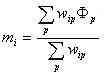
4)Initial Composite
"First Guess". This is how we begin the process.  Since this is an iterative process, we need to jump-start it with something, and this is a composite mixel image using information from all pixel frames.  mixels are computed by tallying "votes" of all pixels that could affect it using a "weighted average" of all pixels from all frames mapped into the mixel coordinate frame.
                .
where
are defined exactly as in step 1, but it is IMPORTANT to note that in general, each coefficient will have to be calculated independently due to the large numbers of pixel-mixel and mixel-pixel calculations involved.

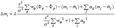
5) Iterative Improvement
                .
where
·regulates the amount that m can change purely for numerical stability
·s is the mixel deviation.  This is typically difficult to deal with.  They mention recalculating it throughout the iterations using representative patches of mixel image
· is the pixel deviation.  Assumed to be the same for all pixels in an image
· ratio of  is the ratio of mixel to pixel deviation

It is easy to see the statistical nature of this method.  Our process is begun by a weighted average to guess the mixel values.  This guess, incidentally, does typically produce good results as Cheeseman noted, but, in Matlab at least, is a very slow thing to compute (though not detrimentally slow.)  In the iterative improvement we can again see the statistical nature.  Note that the top of the equation is composed of

• Sum of weighted pixel differences
• How much the ith mixel deviates from what we expect it to be based on its cardinal neighbors
• Weighted sum of the same value